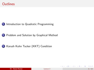
This document provides an overview of quadratic programming, including: 1. It defines quadratic programming as a special case of nonlinear programming where the objective function is quadratic and all constraints are linear. 2. It presents the general mathematical formulation of a quadratic programming problem and provides an example problem. 3. It discusses solutions to quadratic programs using the graphical method and the Karush-Kuhn-Tucker (KKT) conditions.

1. Quadratic Programming
Dr. Varun Kumar
Dr. Varun Kumar Lecture 2 1 / 12

2. Outlines
1 Introduction to Quadratic Programming
2 Problem and Solution by Graphical Method
3 Karush Kuhn Tucker (KKT) Condition
Dr. Varun Kumar Lecture 2 2 / 12

3. Introduction to Quadratic Programming
⇒ Quadratic programming problem (QPP) is special case of non-linear
programming problem (NLPP).
⇒ Objective function is quadratic in nature.
⇒ All constraints (in-equality and equality) are linear in nature.
⇒ General mathematical formulation for QPP
min{f (x)} =xT
Qx + cT
x
s.t Ax ≤ b
x ≥ 0
⇒ Q = [qij ]n×n → Symmetric positive semi-definite matrix.
⇒ c, x ∈ Rn → Vector of size n × 1 (Contain real number).
⇒ A = [aij ]m×n → Matrix of size m × n
Dr. Varun Kumar Lecture 2 3 / 12

4. Example:
⇒ Let objective function f (x) = 3x2
1 + 4x2
2 + 2x1x2 − 2x1 − 3x2
⇒ Constraint:
3x1 + 2x2 ≤ 6
x1 + x2 ≤ 2
x1, x2 ≥ 0
⇒ Problem representation
min{f (x)} = [x1 x2]
3 1
1 4
x1
x2
+ [−2 − 3]
x1
x2
3 2
1 1
x1
x2
≤
6
2
⇒ x =
x1
x2
, Q =
3 1
1 4
, b =
6
2
, A =
3 2
1 1
, c =
−2
−3
Dr. Varun Kumar Lecture 2 4 / 12

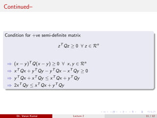
5. Solution by the graphical method:
Positive semi-definite and symmetric
⇒ Q =
3 1
1 4
→ [qij ]2×2, if qij = qji → Symmetric
⇒ If det|Q| ≥ 0 → Positive semi-definite
Solution by graphical method:
⇒ Let objective function f (x) = (x1 − 2)2 + (x2 − 1)2
⇒ Constraint:
x1 + x2 ≤ 2
x1, x2 ≥ 0
Dr. Varun Kumar Lecture 2 5 / 12

6. Karush Kuhn Tucker KKT condition:
QPP should be written in this form
⇒ min{f (x)} = xT
Qx + cT
x
⇒ Ax ≤ b (1)
⇒ −x ≤ 0 (2)
Let KKT multiplier associated with the constraints (1) and (2) be u ∈ Rm
and v ∈ Rn, respectively. Hence,
cT
+ 2xT
Q + uT
A − vT
= 0
uT
(Ax − b) − vT
x = 0
Ax − b = 0
x ≥ 0, u ≥ 0, v ≥ 0
Note: Total number of KKT multiplier for solving QPP is m + n.
Dr. Varun Kumar Lecture 2 6 / 12

7. General KKT condition
General KKT condition
⇒ ∇f (x) +
PN
i=1 λi ∇gi (x) = 0
⇒ λi gi (x) = 0 ∀ i
⇒ gi (x) ≤ 0
⇒ λi ≥ 0
Here,
∇f (x) =
∂f (x)
∂x1
,
∂f (x)
∂x2
, ......,
∂f (x)
∂xn
Example
⇒ f (x) = 3x2
1 + 2x2
2 + x1x2 − 4x1 − 2x2
s.t x1 + 2x2 ≤ 6 → u
−x1 ≤ 0 → v1
−x2 ≤ 0 → v2
Dr. Varun Kumar Lecture 2 7 / 12

8. Continued–
As per the question f (x) = 3x2
1 + 2x2
2 + x1x2 − 4x1 − 2x2, s.t
x1 + 2x2 ≤ 6 → u, −x1 ≤ 0 → v1, −x2 ≤ 0 → v2. Hence,
Applying KKT condition:
6x1 + x2 − 4, 4x2 + x1 − 2
+ u 1, 2
+ v1(−1, 0) + v2(0, −1) = (0, 0)
6x1 + x2 − 4 + u − v1 = 0
x1 + 4x2 − 2 + 2u − v2 = 0
General KKT condition for QPP
2xT
Q + cT
+ uT
A + vT
(−I) = 0
uT
(Ax − b) − vT
x = 0
Ax − b ≤ 0
x ≥ 0, u ≥ 0, v ≥ 0
Dr. Varun Kumar Lecture 2 8 / 12

9. Continued–
Taking transpose operation in 1st KKT expression
2Qx + c + AT
u + v(−I) = 0
uT
(Ax − b) − vT
x = 0
Ax − b + s = 0
x ≥ 0, u ≥ 0, v ≥ 0
Here, 0s0 is called as the slack variable. ⇒ uT (−s) − vT x = 0
⇒ uT s = 0 ⇒ u1s1 + u2s2 + ... + umsm = 0
⇒ ; vT x = 0 ⇒ v1x1 + v2x2 + ..... + vnxn = 0
⇒ ui si = 0 ∀ i = 1, 2, ...., m and vj xj = 0 ∀ j = 1, 2, ...n




2Qx + c + AT u − v = 0
Ax + s = b
ui si = 0 ∀ i = 1, 2, ...., m
vj xj = 0 ∀ j = 1, 2, ...n




Dr. Varun Kumar Lecture 2 9 / 12

10. Continued–
The matrix form of KKT conditions are
2Q AT In 0
A 0 0 In




x
u
v
s




−c
b
Theorem
Let Q be a +ve semi-definite matrix of order n. Then for any x, y ∈ Rn
2xT
Qy ≤ xT
Qx + yT
Qy
Problem: Show that f (x) = xT Qx + cT x, x ∈ Rn (in QPP) is a convex
function, if Q is a semi-definite symmetric matrix.
Dr. Varun Kumar Lecture 2 10 / 12

11. Continued–
Condition for +ve semi-definite matrix
zT
Qz ≥ 0 ∀ z ∈ Rn
⇒ (x − y)T Q(x − y) ≥ 0 ∀ x, y ∈ Rn
⇒ xT Qx + yT Qy − yT Qx − xT Qy ≥ 0
⇒ yT Qx + xT Qy ≤ xT Qx + yT Qy
⇒ 2xT Qy ≤ xT Qx + yT Qy
Dr. Varun Kumar Lecture 2 11 / 12

12. Dr. Varun Kumar Lecture 2 12 / 12