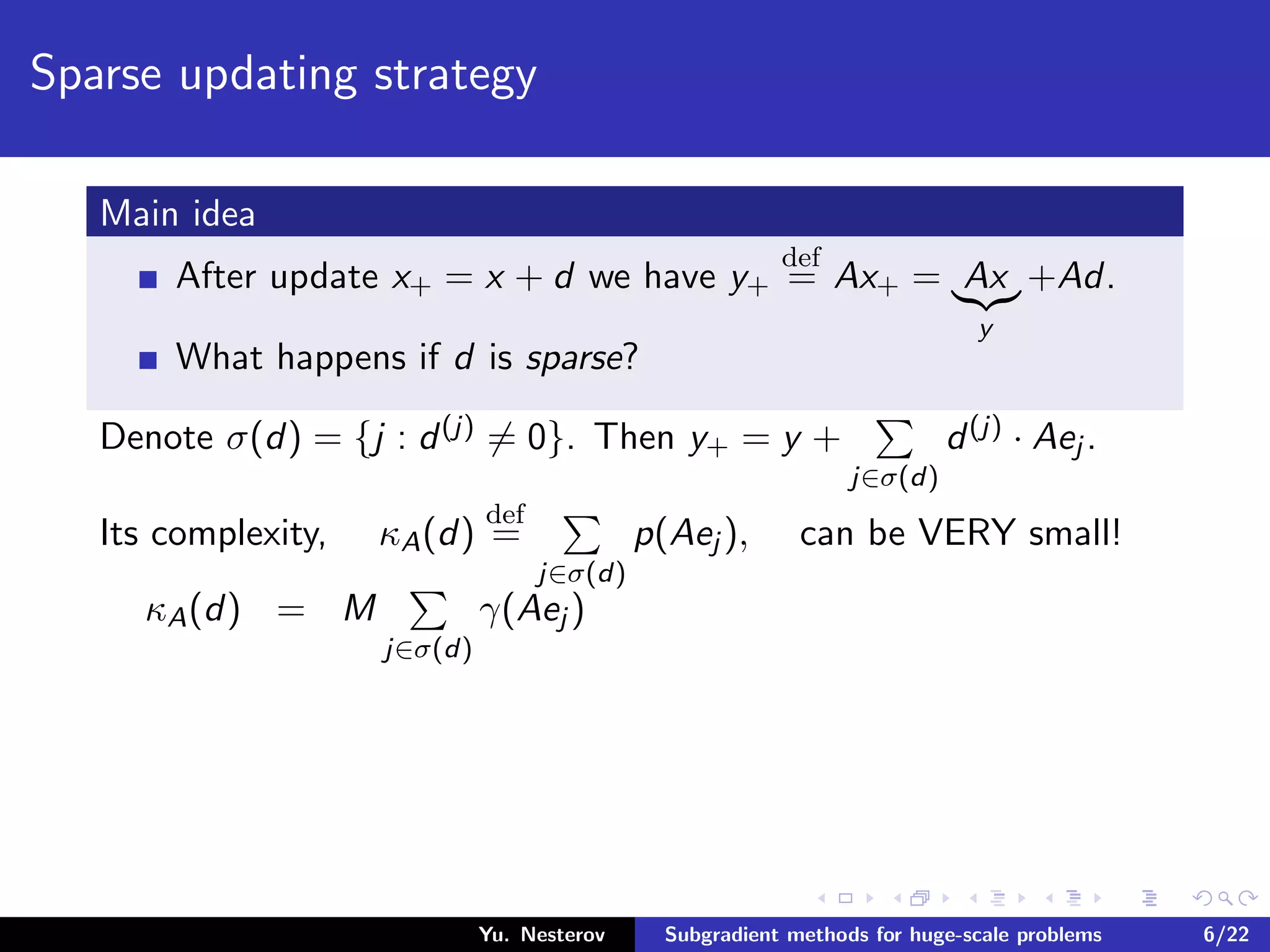
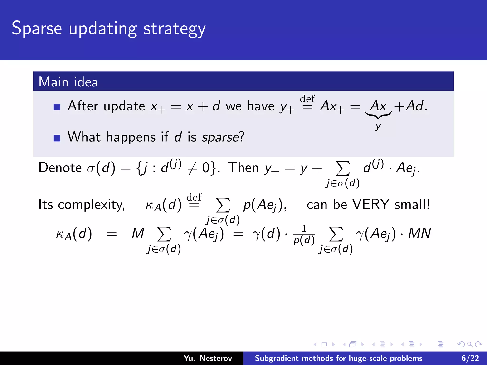
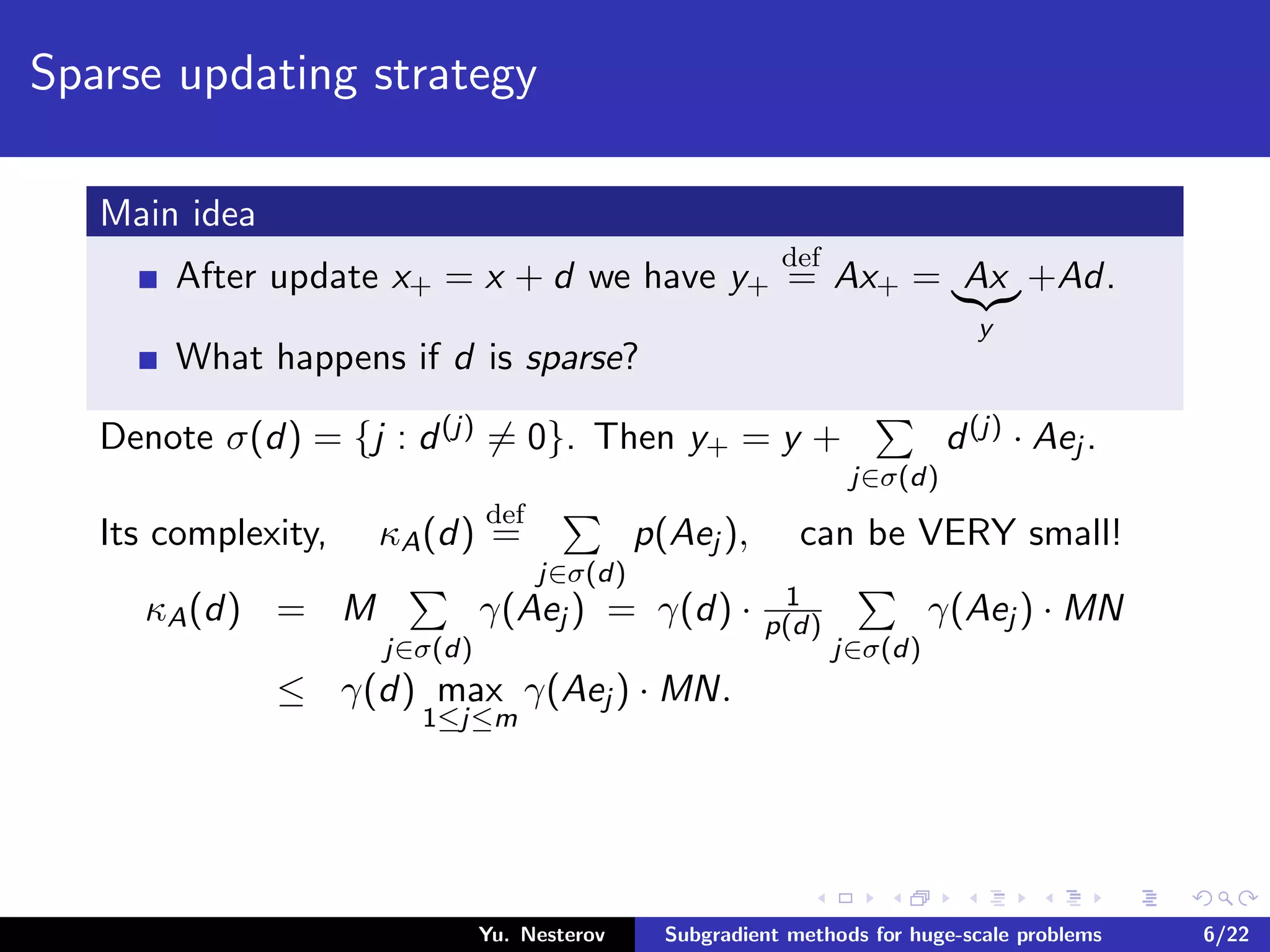
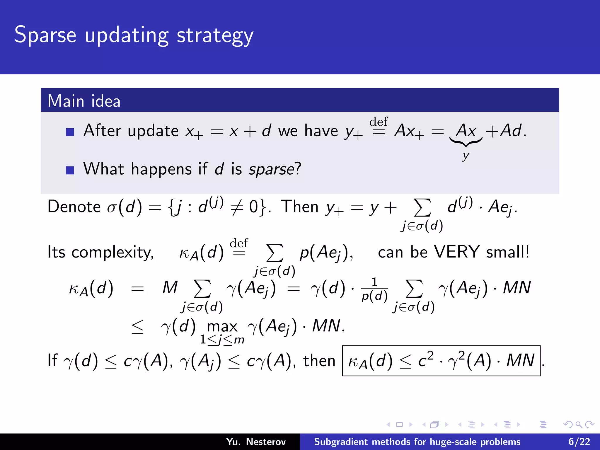
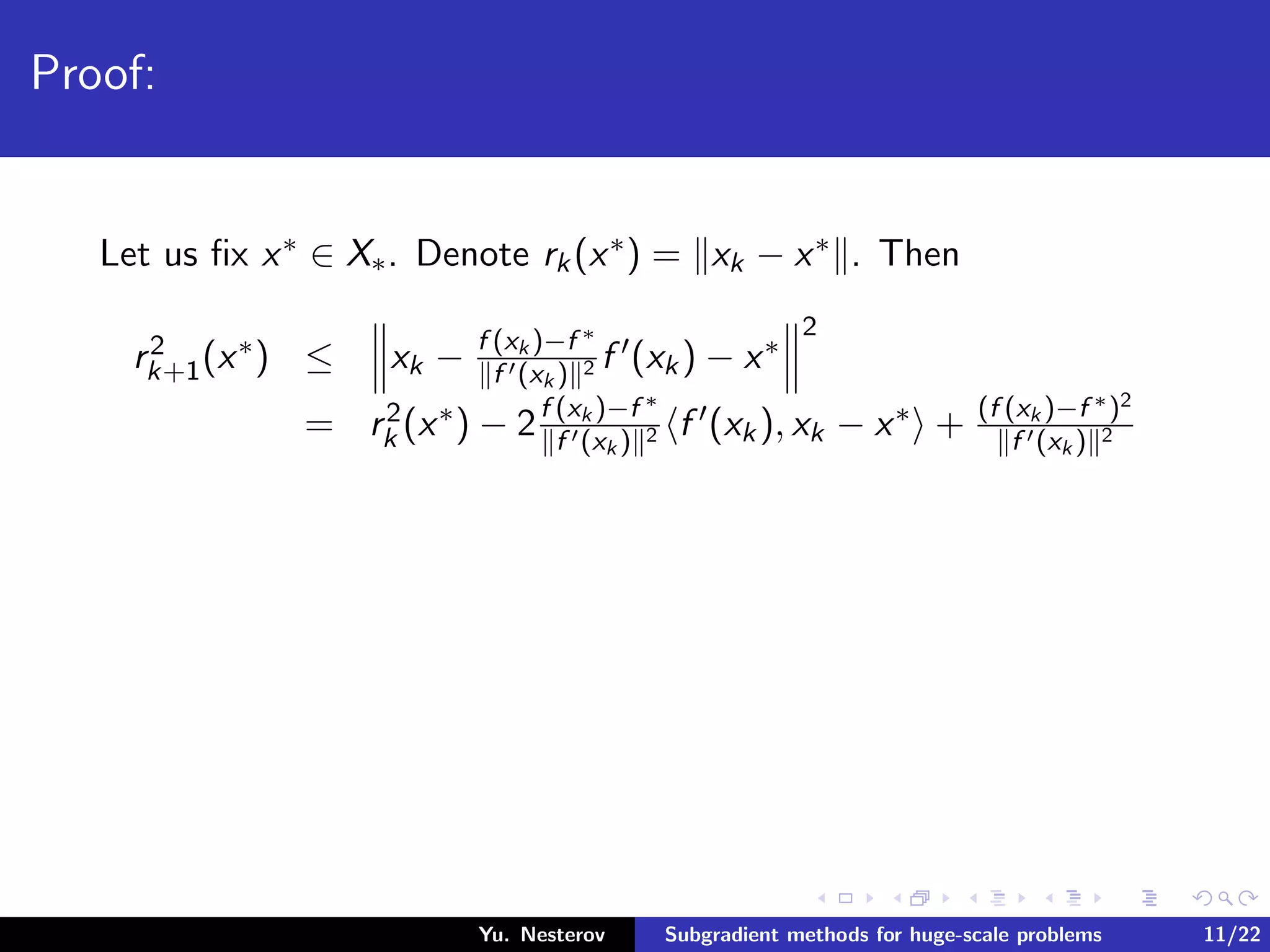
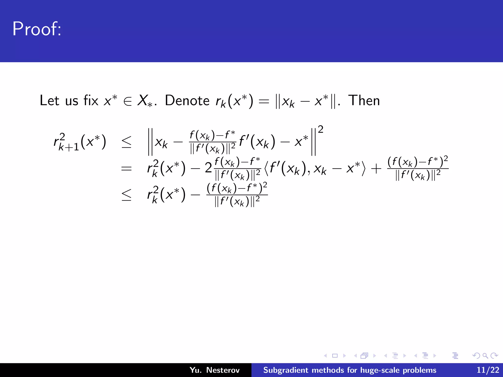
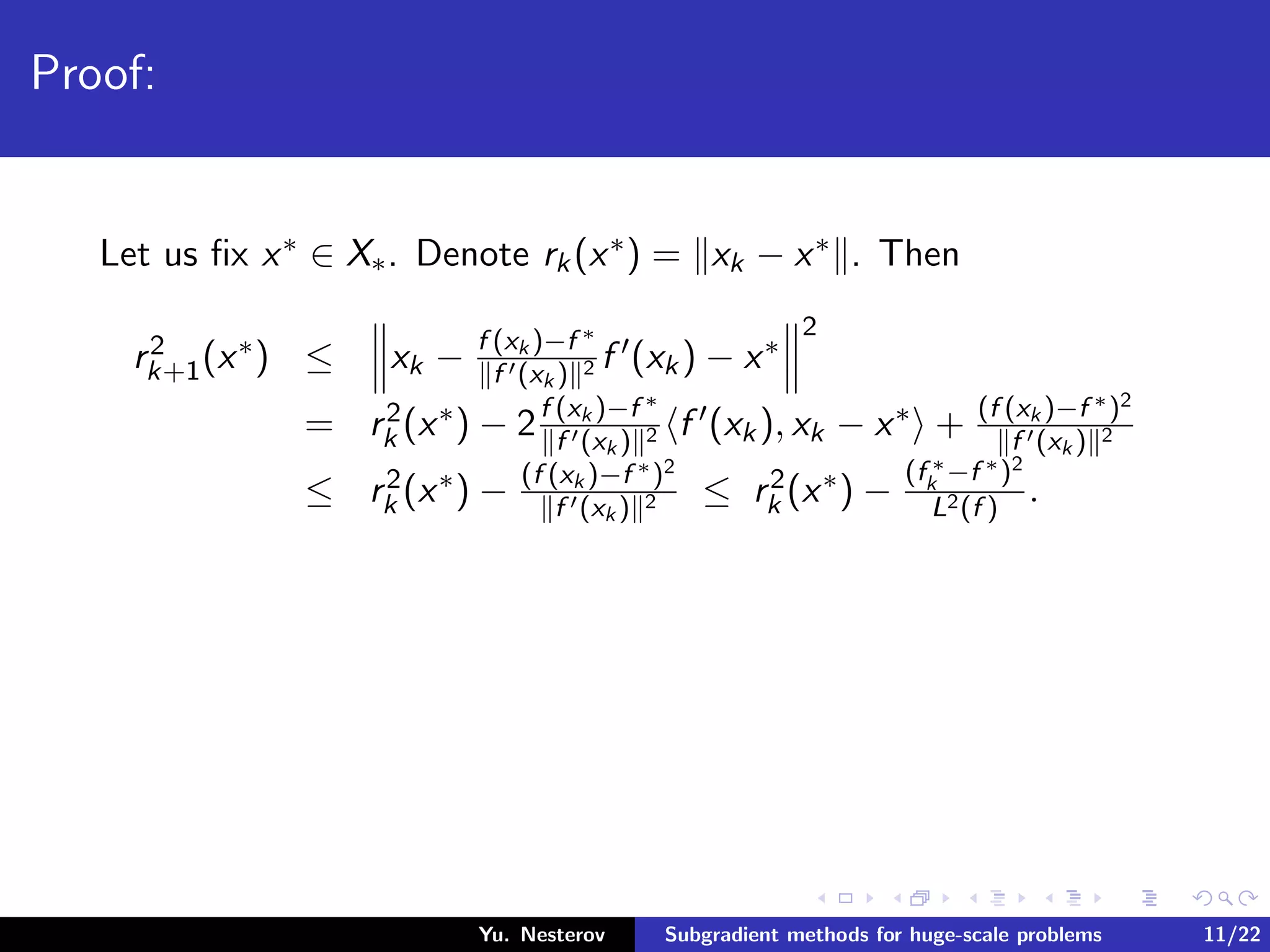
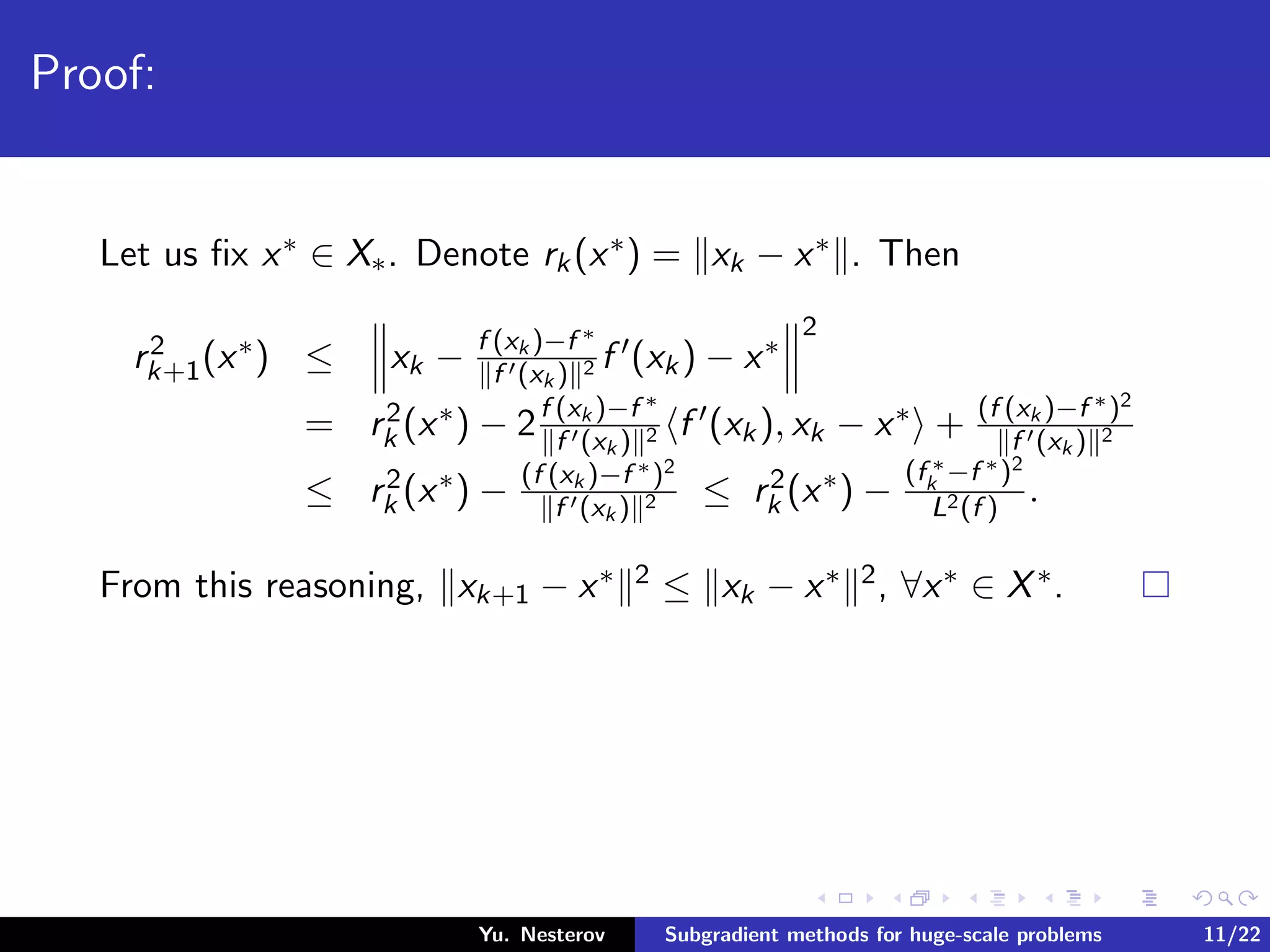
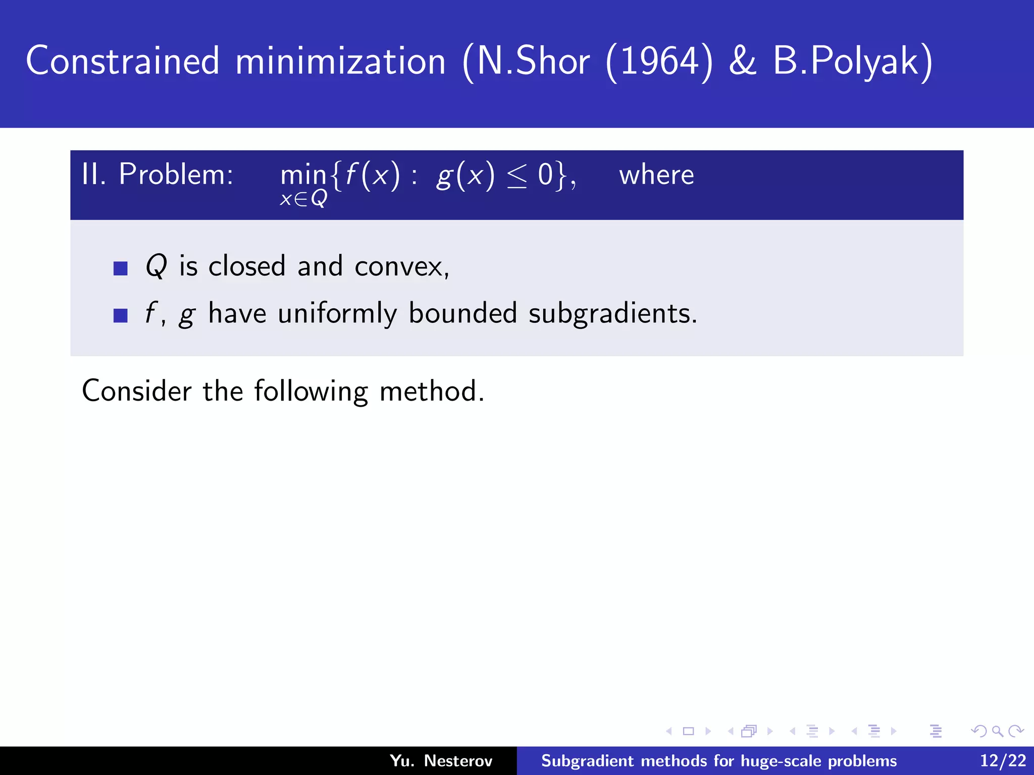
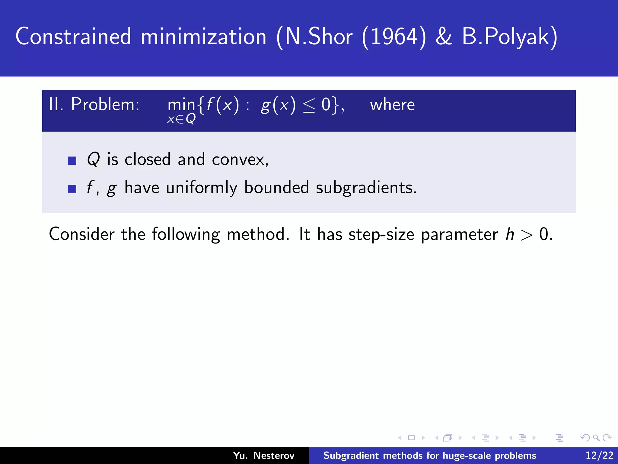
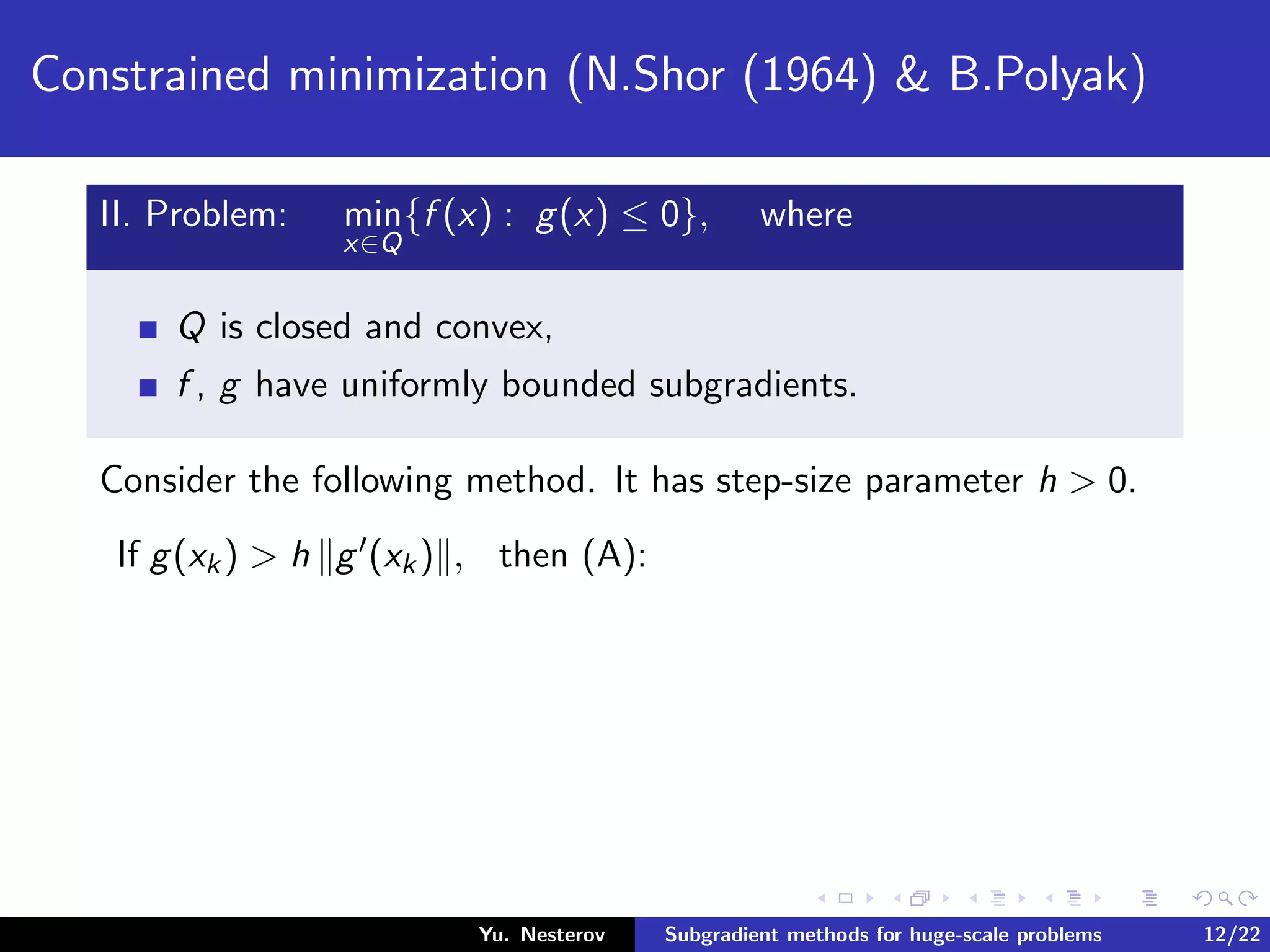
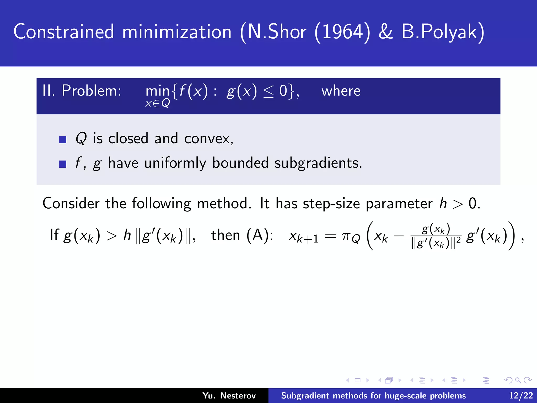
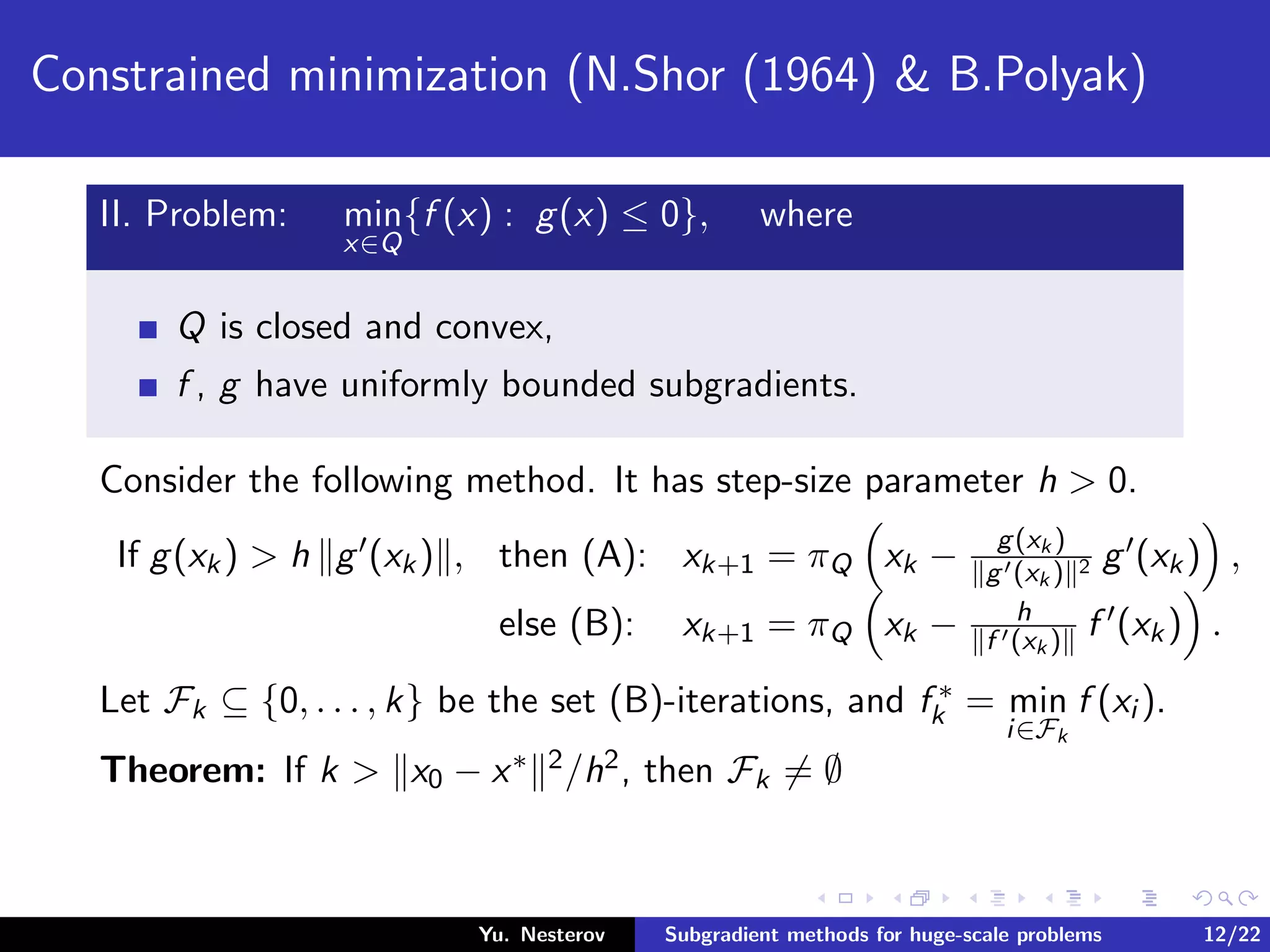
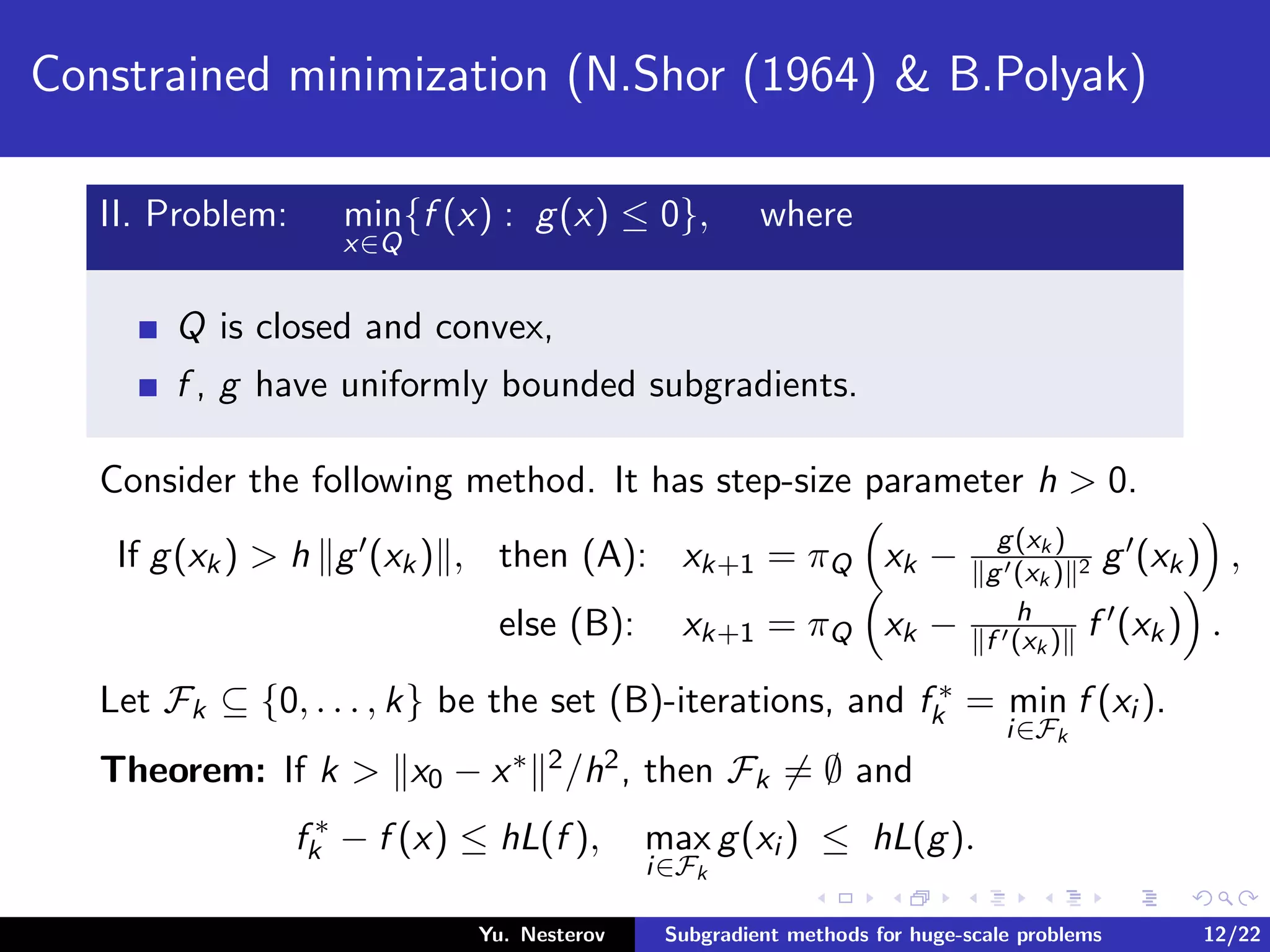
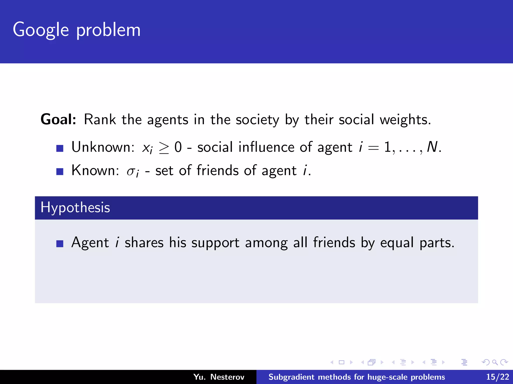
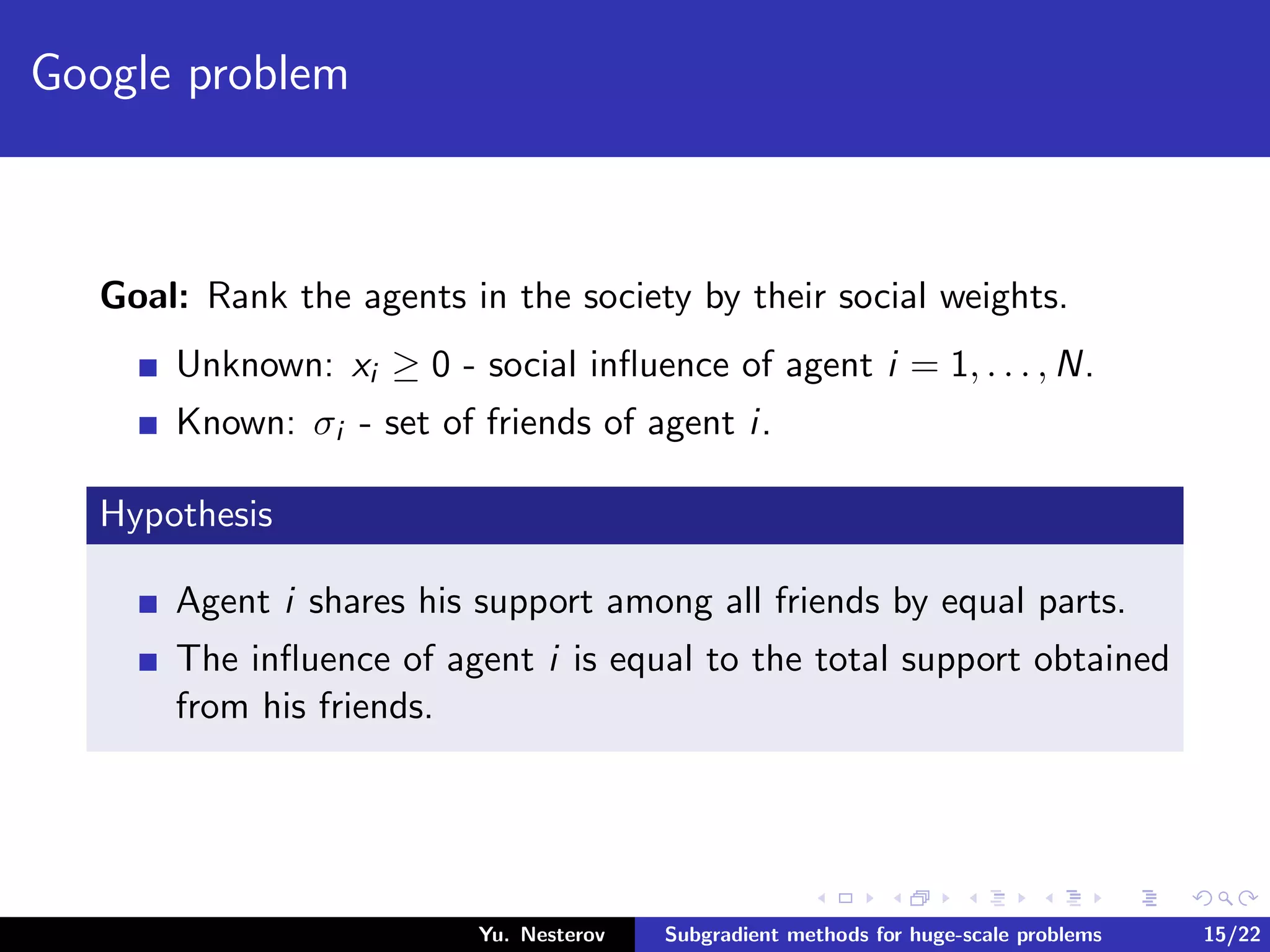
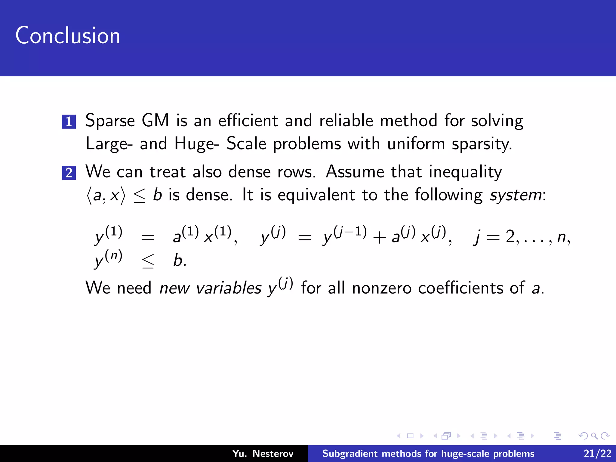
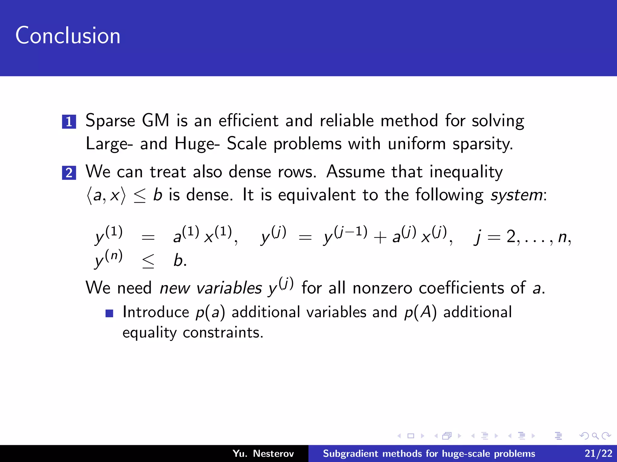
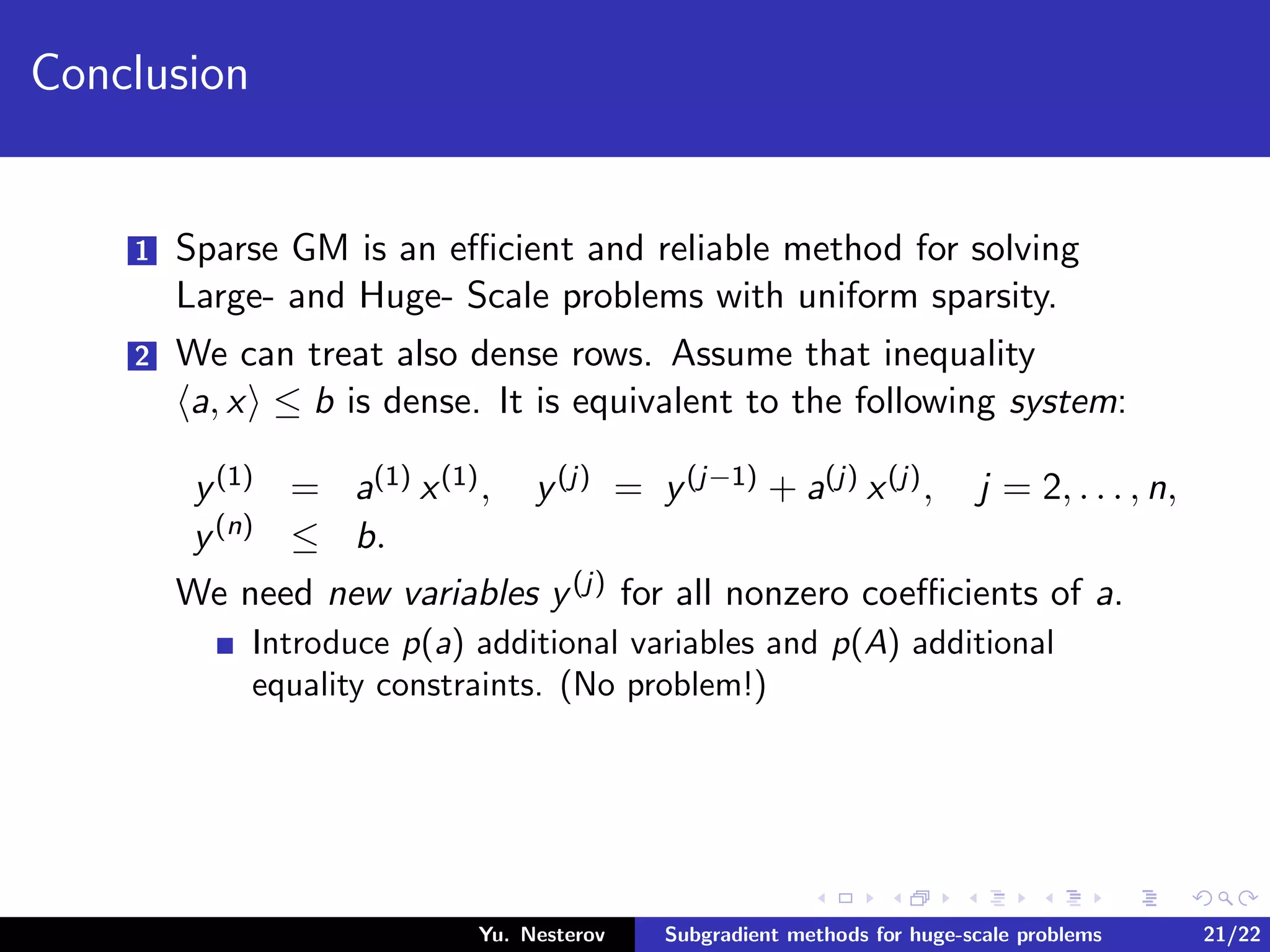
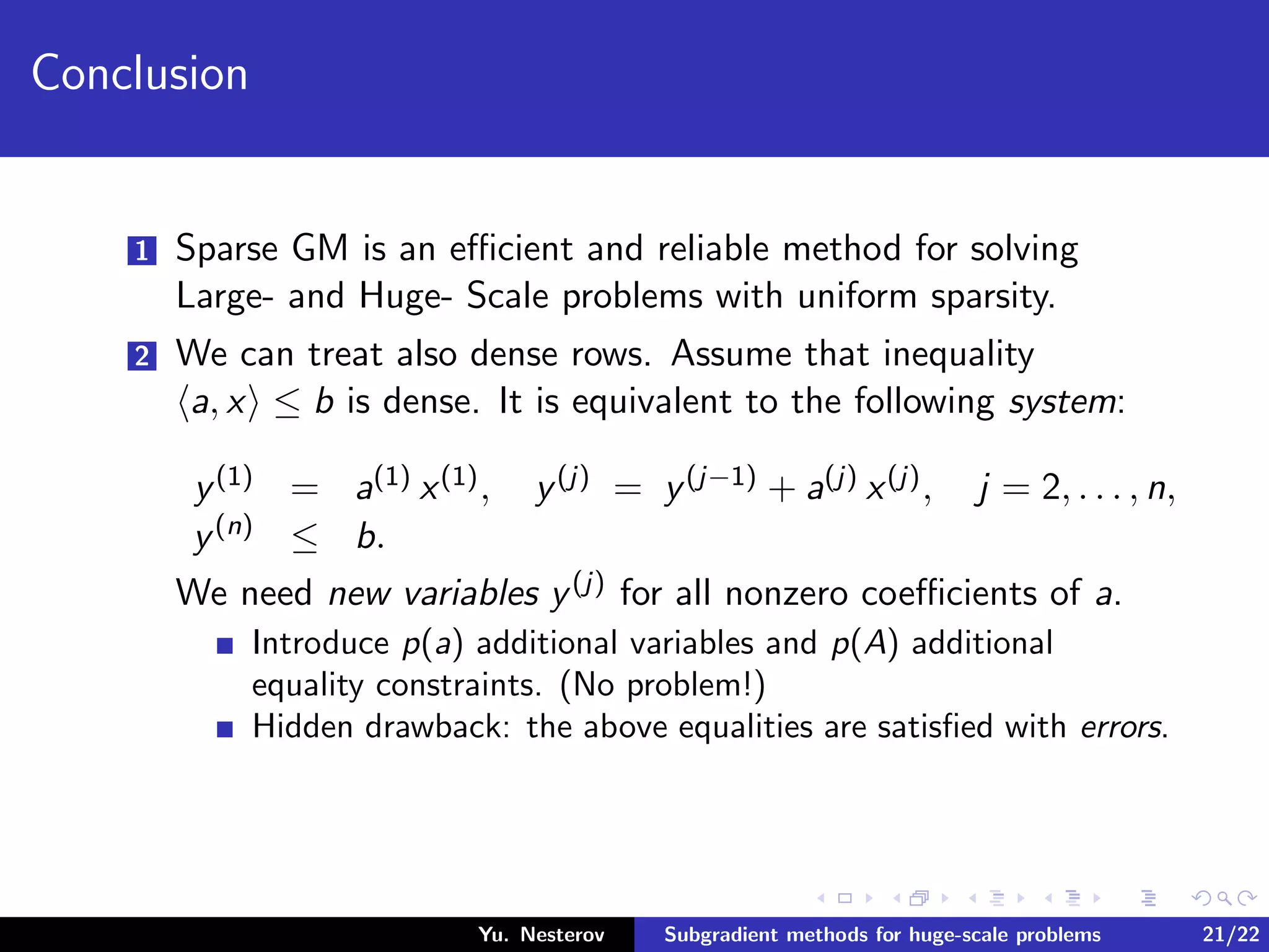
Download as PDF, PPTX
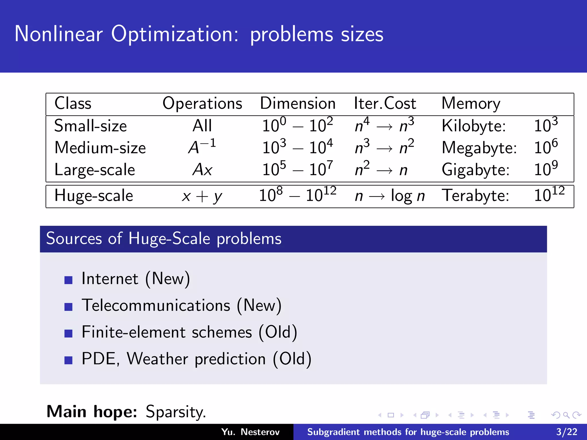
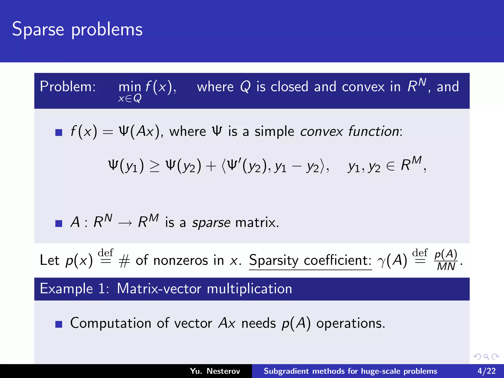


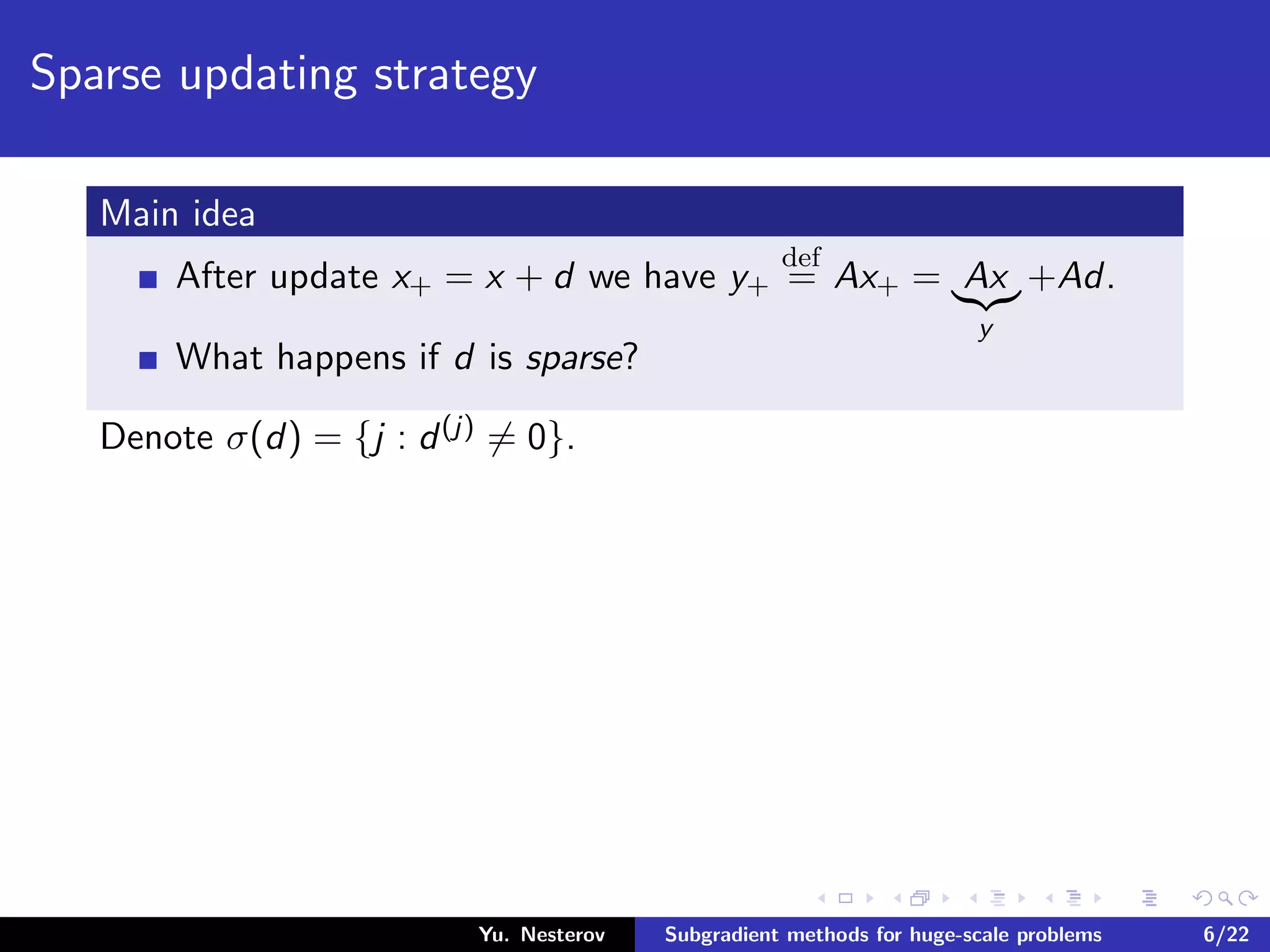
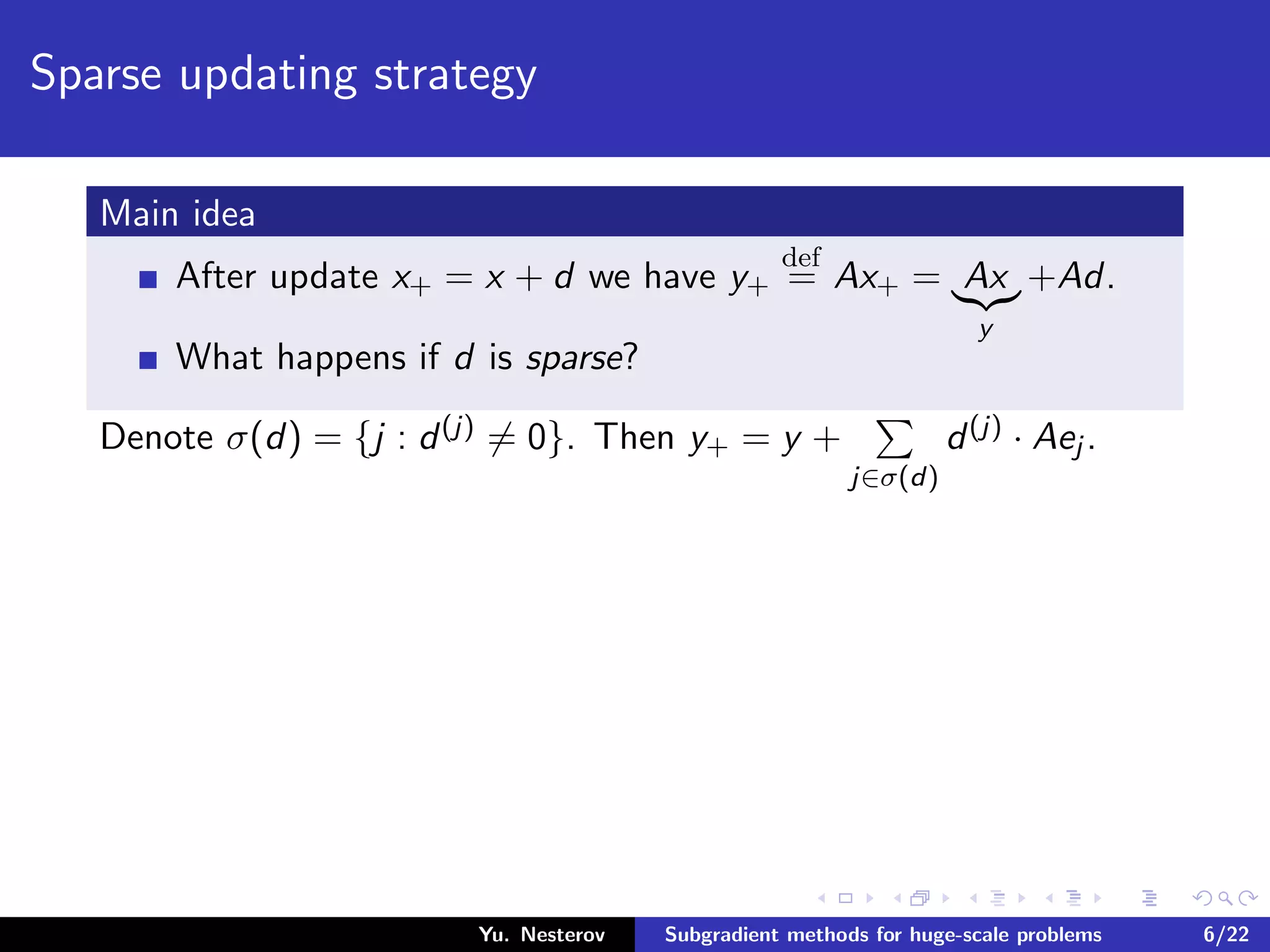
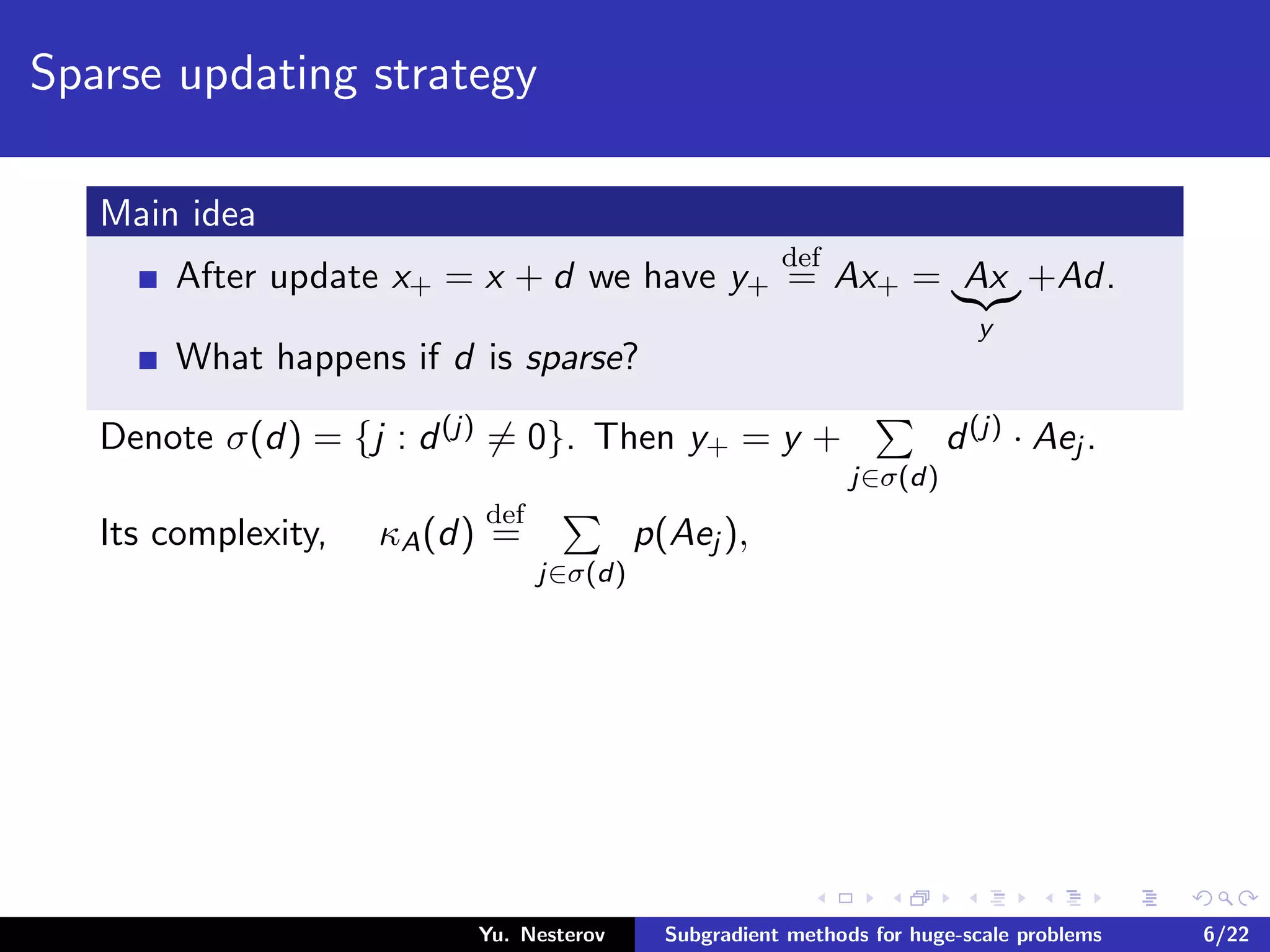
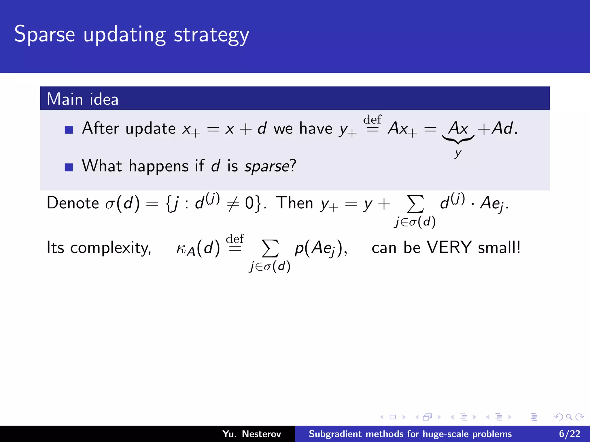


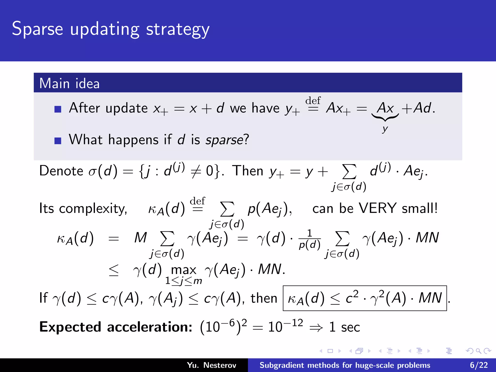
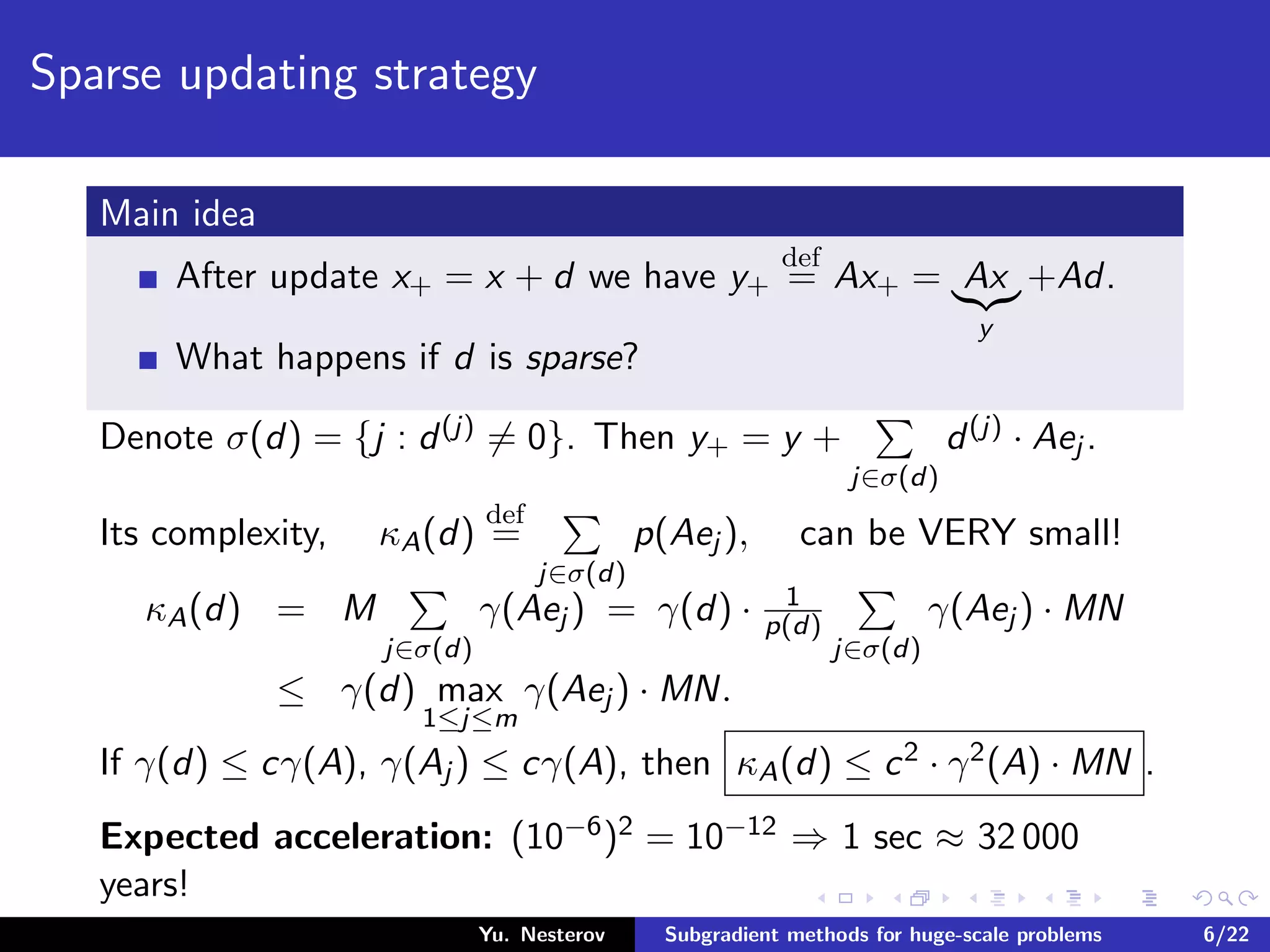


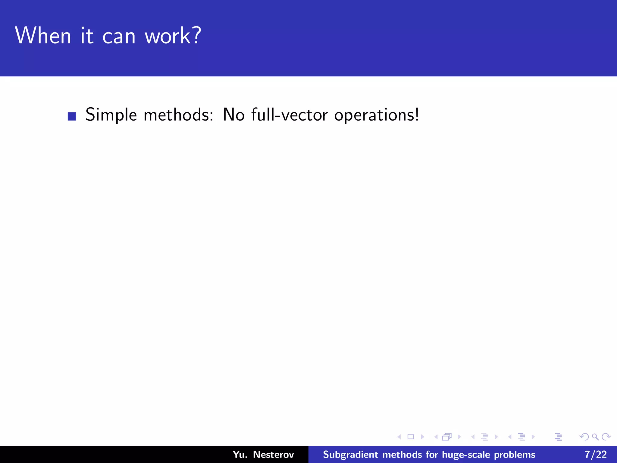
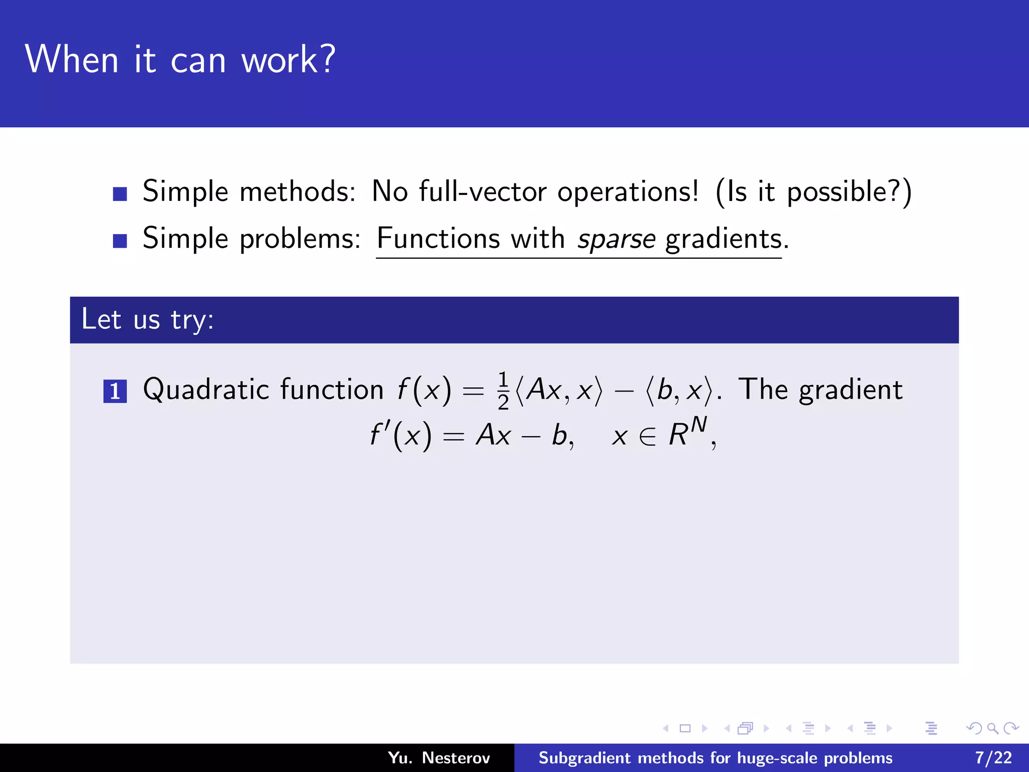
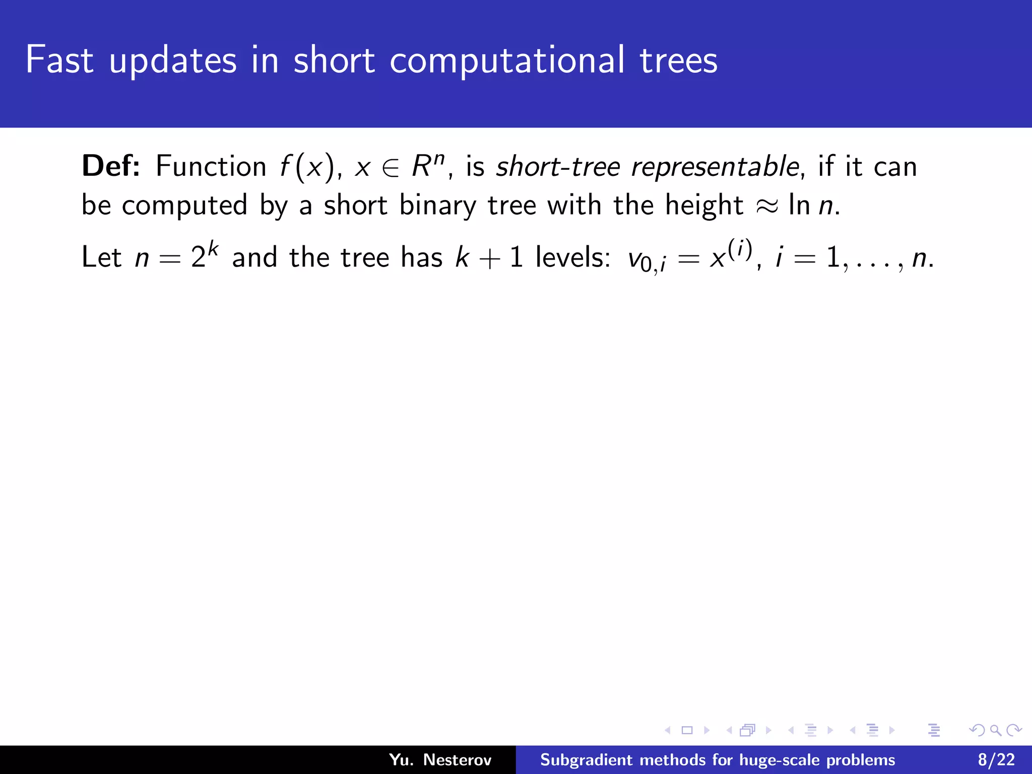
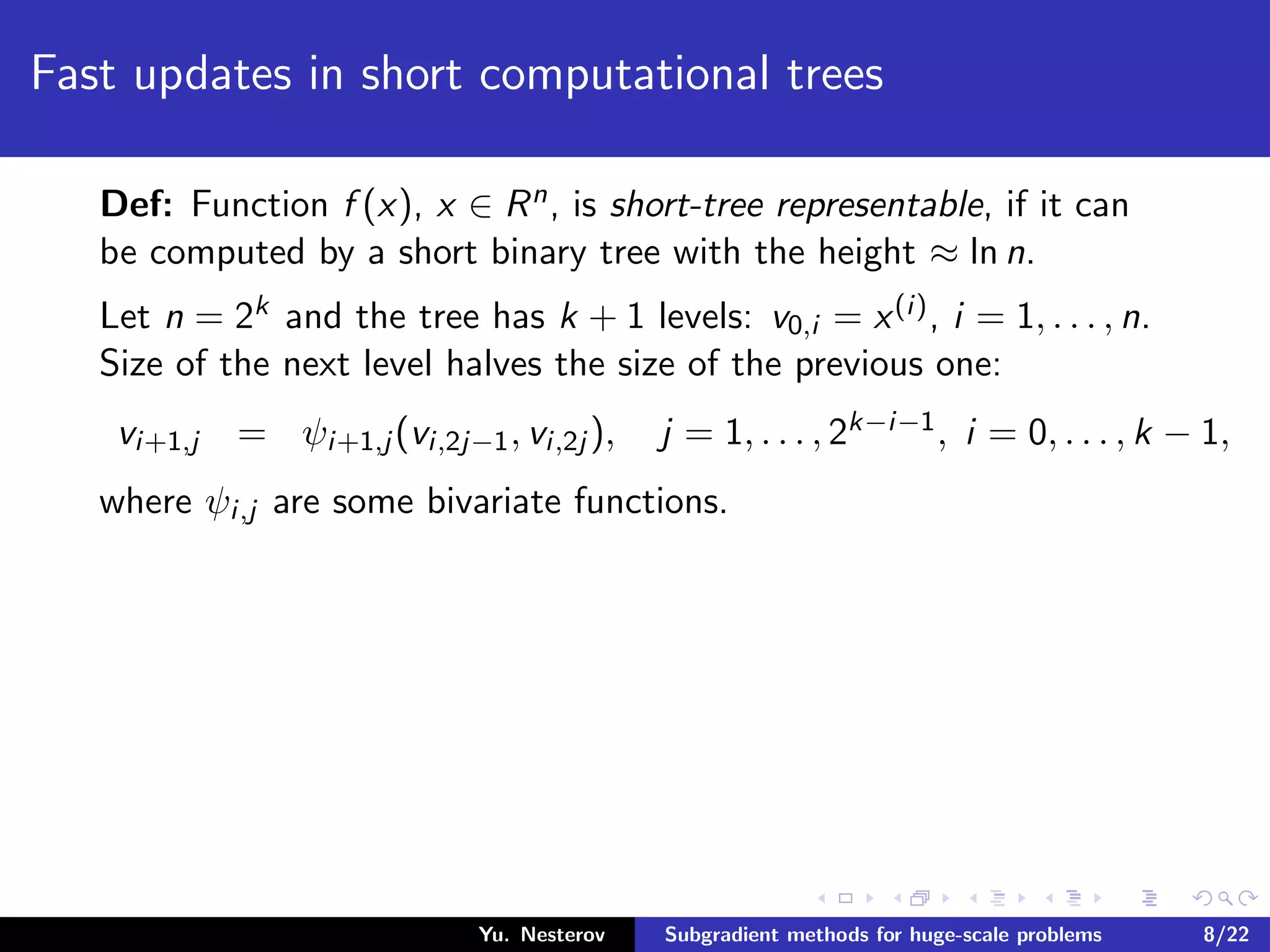
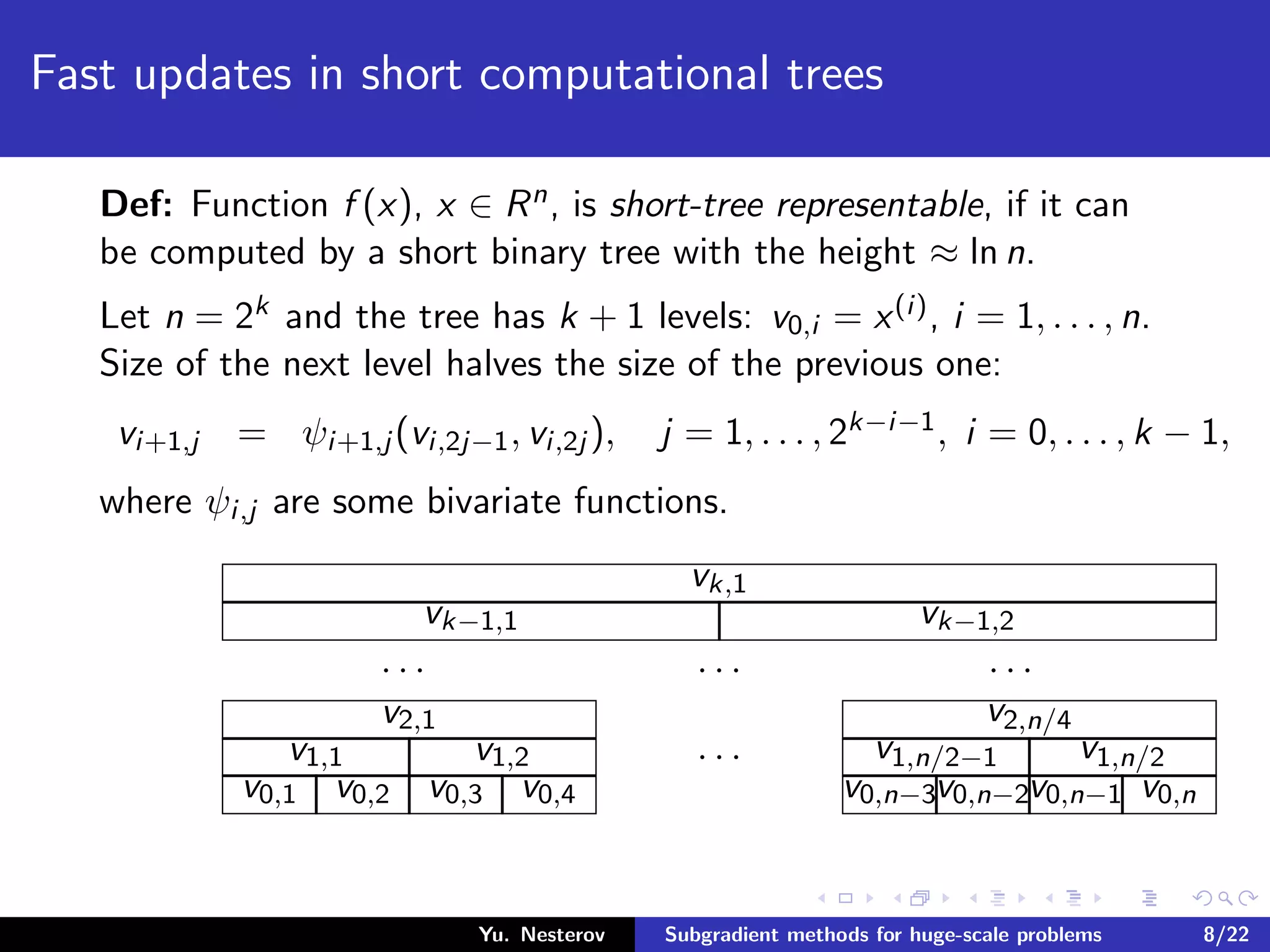
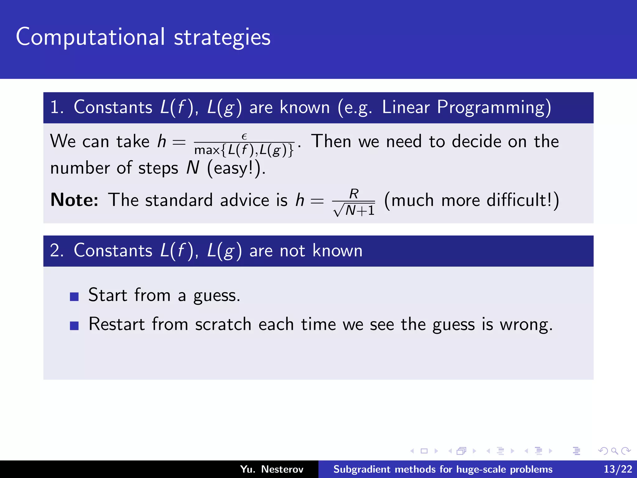
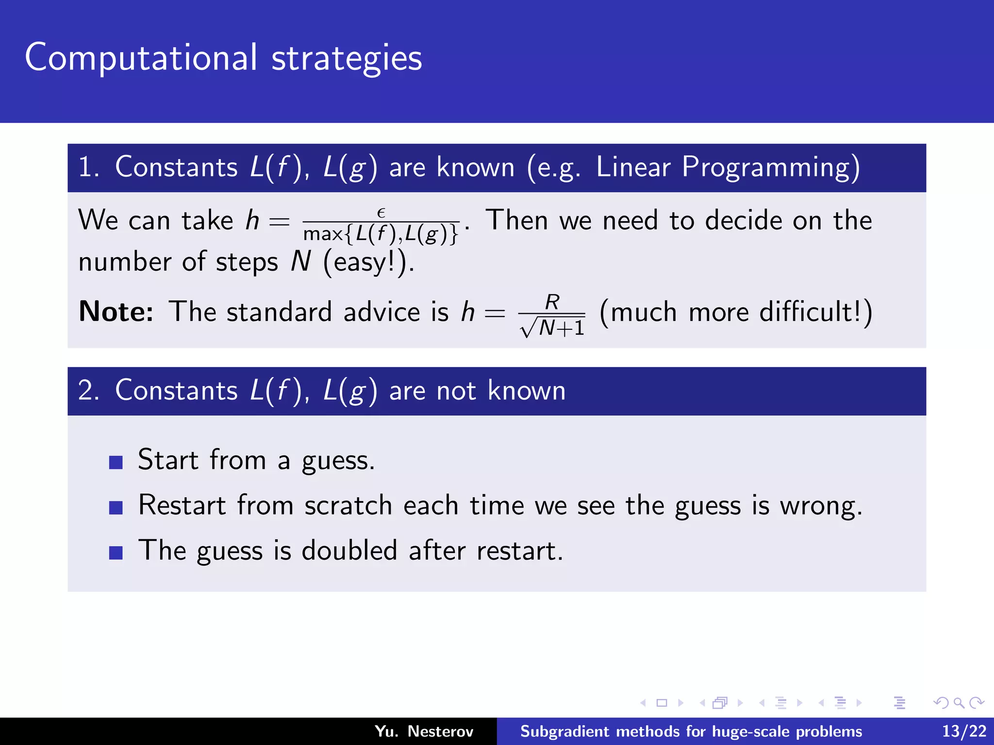
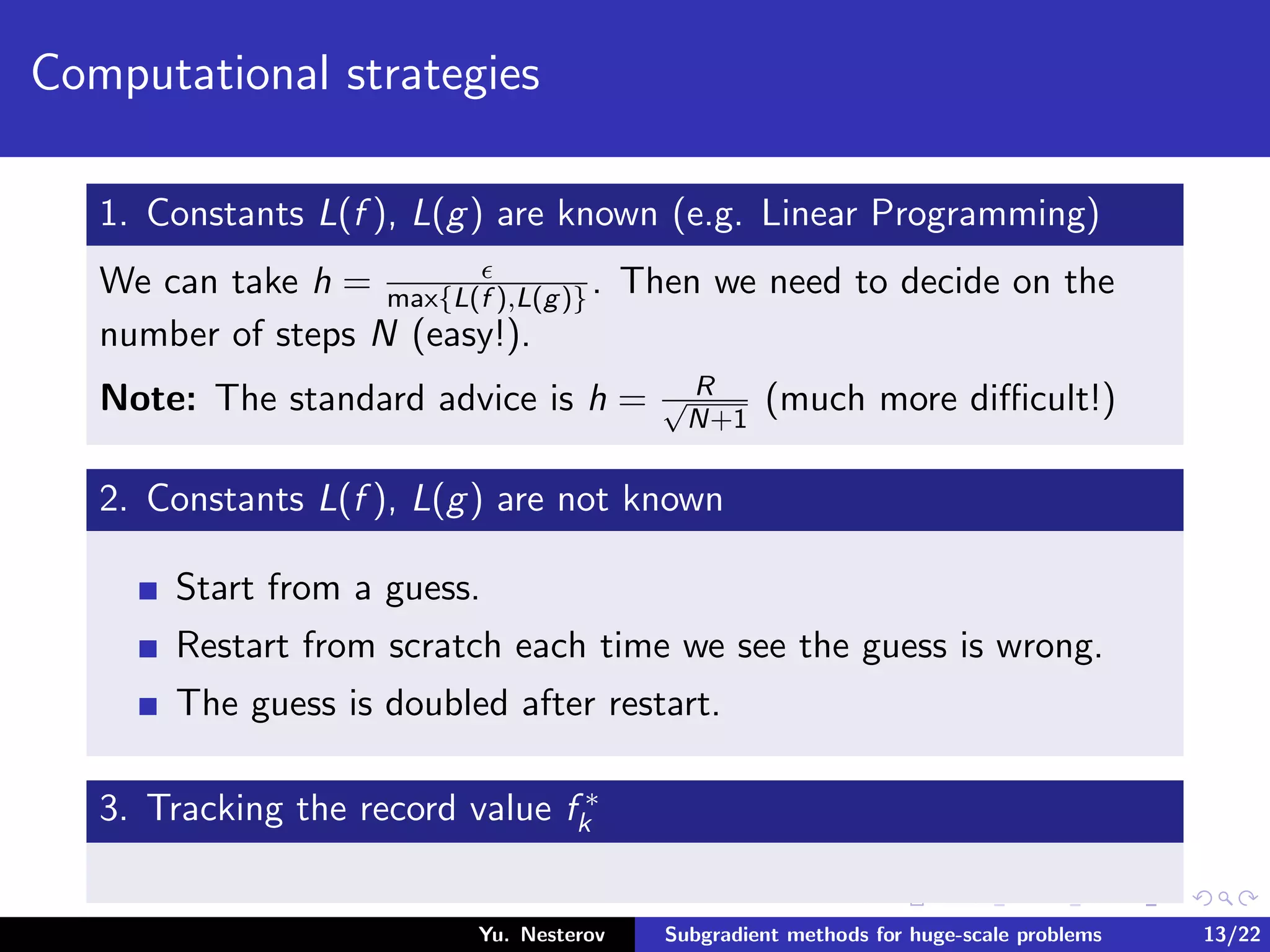
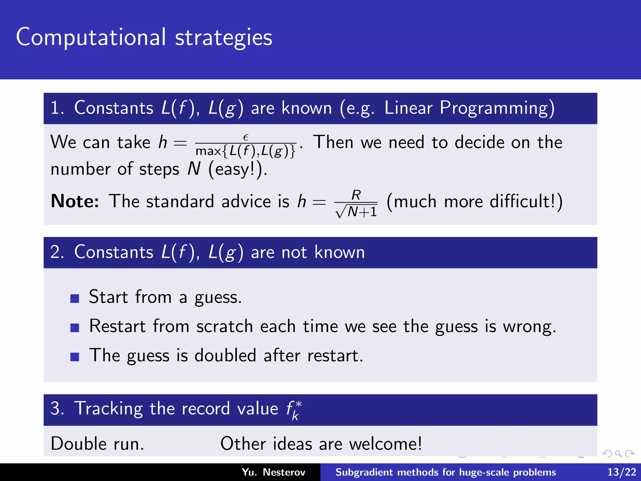
![When it can work?
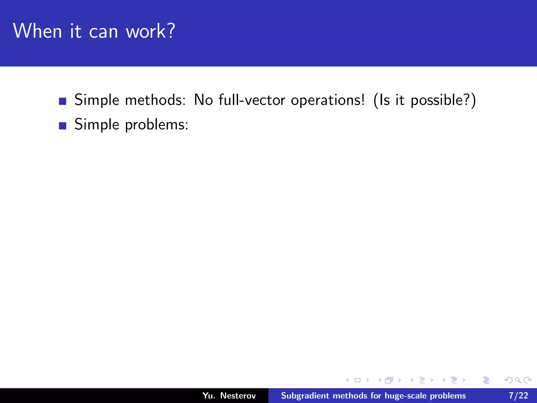
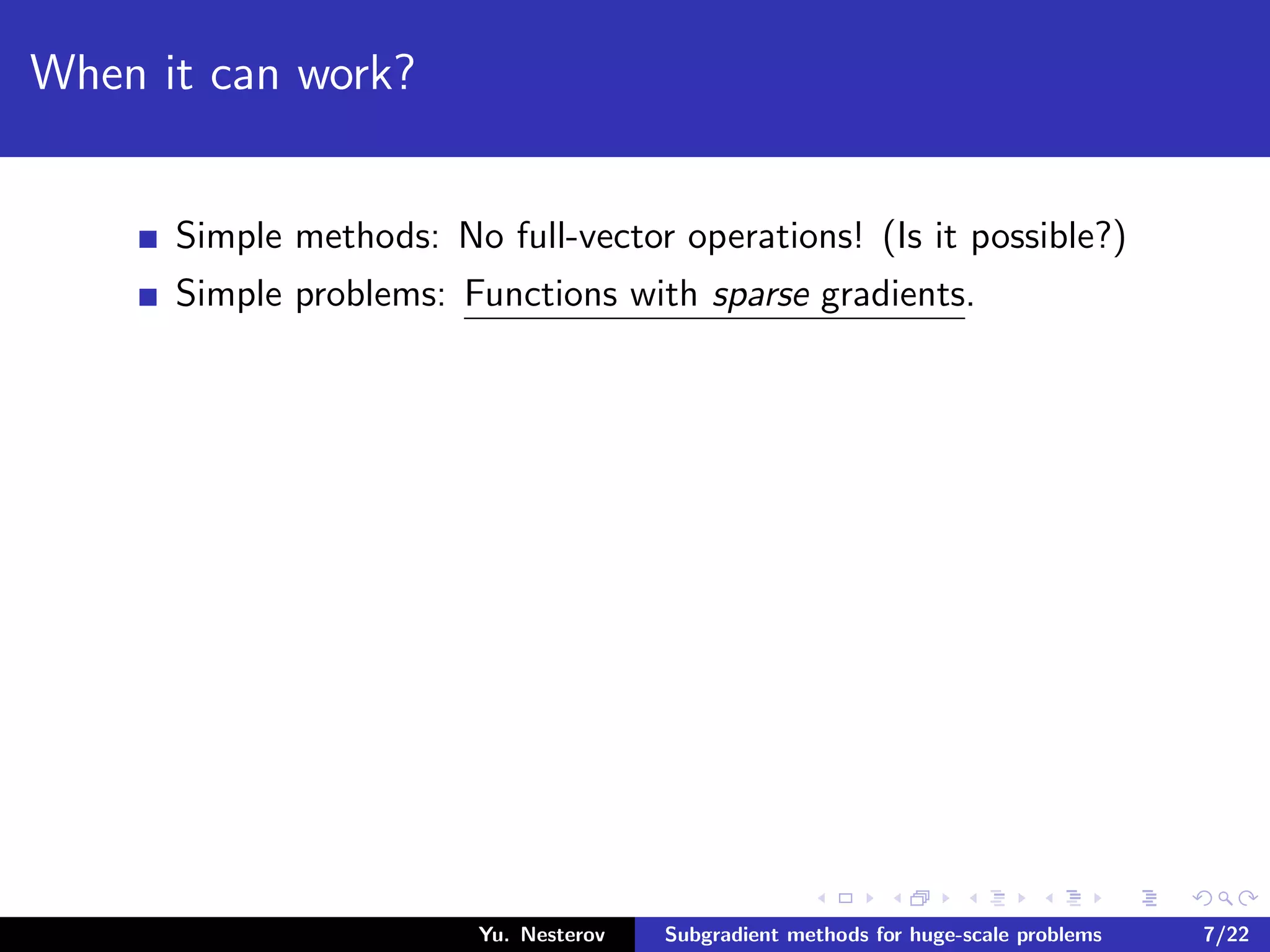
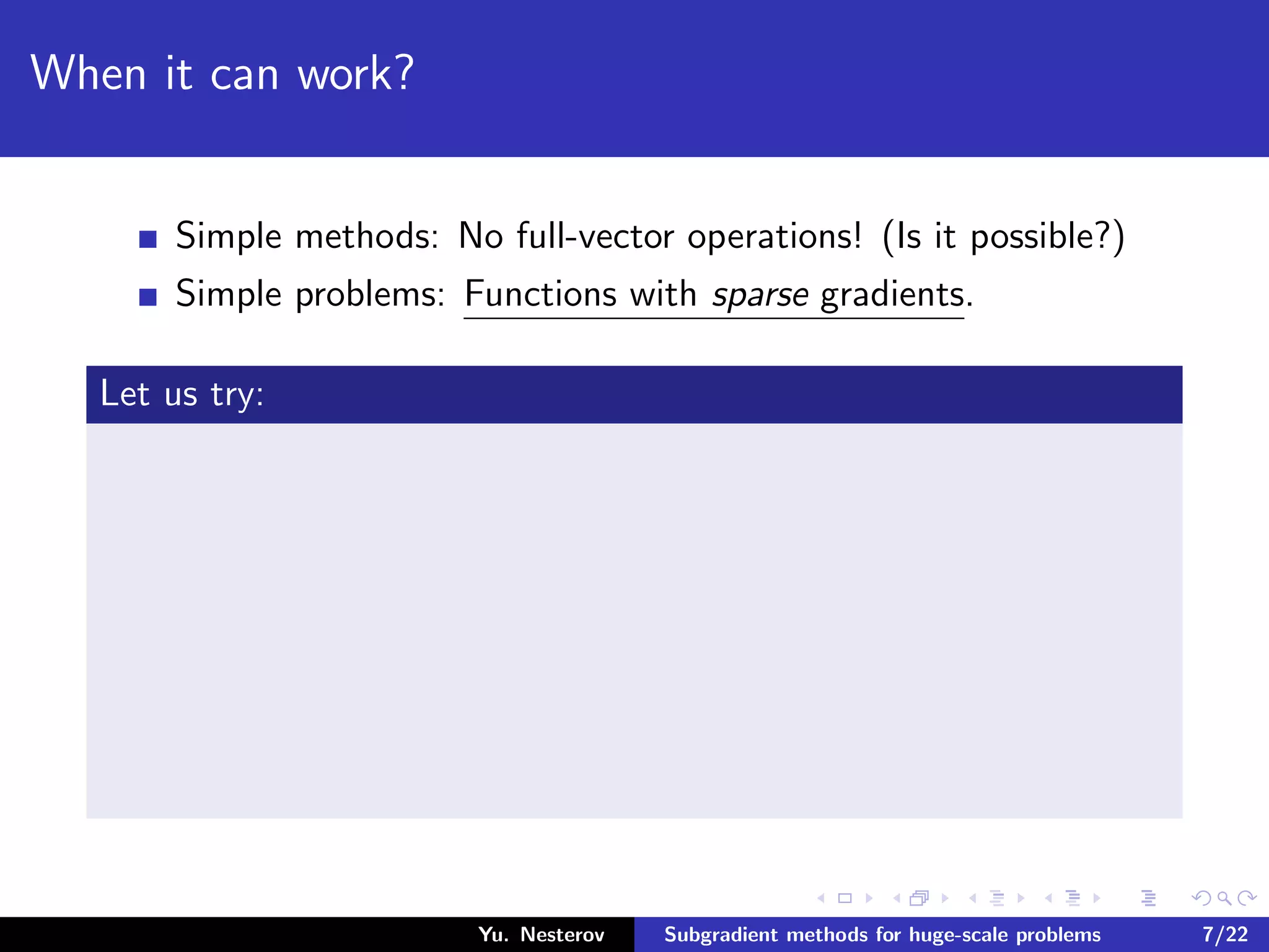
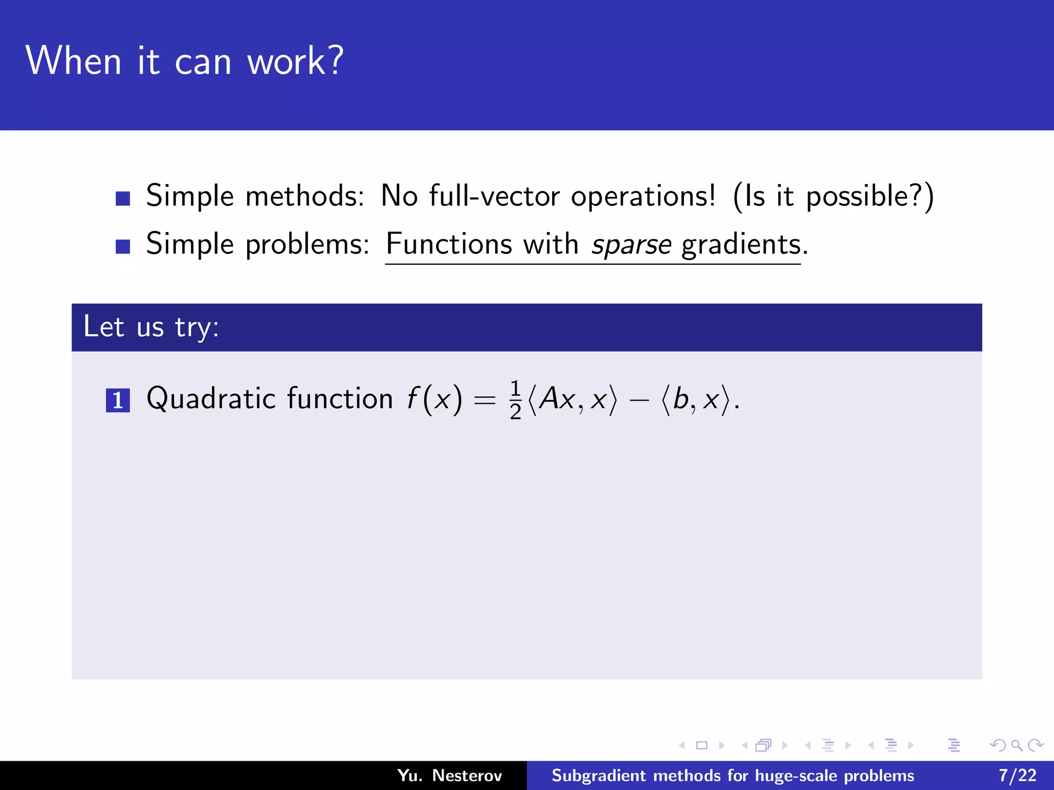
Simple methods: No full-vector operations! (Is it possible?)
Simple problems: Functions with sparse gradients.
Let us try:
1 Quadratic function f (x) = 1
2 Ax, x − b, x . The gradient
f (x) = Ax − b, x ∈ RN
,
is not sparse even if A is sparse.
2 Piece-wise linear function g(x) = max
1≤i≤m
[ ai , x − b(i)].
Yu. Nesterov Subgradient methods for huge-scale problems 7/22](https://image.slidesharecdn.com/sublinbm1-141114054915-conversion-gate02/75/Subgradient-Methods-for-Huge-Scale-Optimization-Problems-Catholic-University-of-Louvain-Belgium-59-2048.jpg)
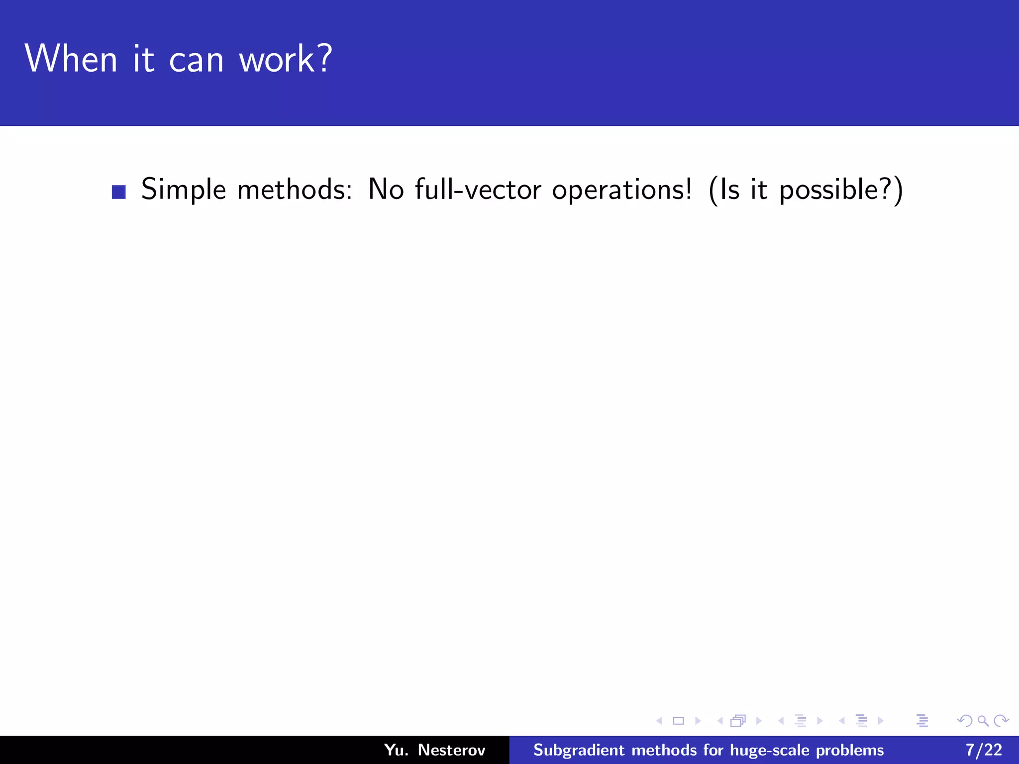
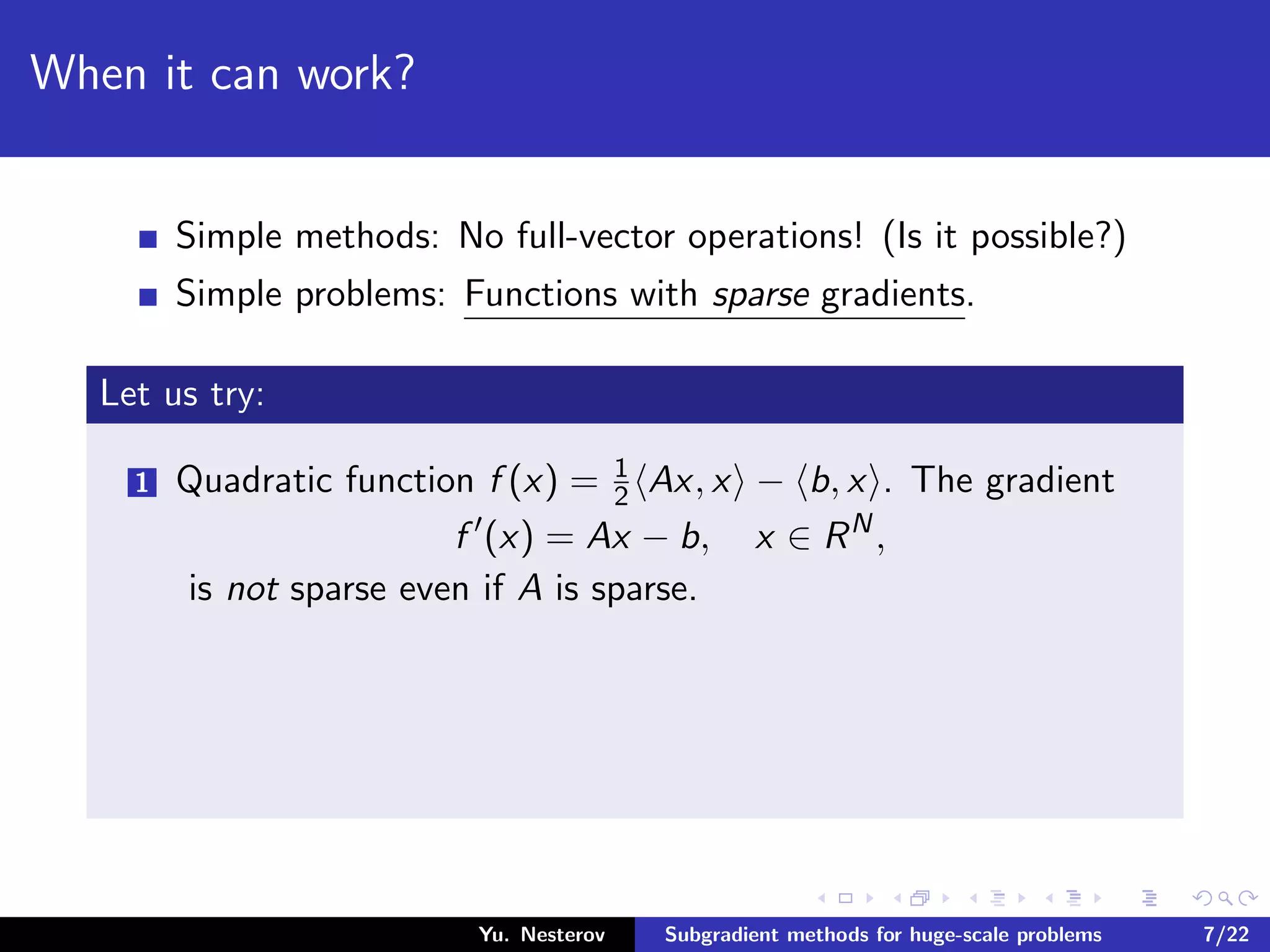
![When it can work?
Simple methods: No full-vector operations! (Is it possible?)
Simple problems: Functions with sparse gradients.
Let us try:
1 Quadratic function f (x) = 1
2 Ax, x − b, x . The gradient
f (x) = Ax − b, x ∈ RN
,
is not sparse even if A is sparse.
2 Piece-wise linear function g(x) = max
1≤i≤m
[ ai , x − b(i)]. Its
subgradient f (x) = ai(x), i(x) : f (x) = ai(x), x − b(i(x)),
Yu. Nesterov Subgradient methods for huge-scale problems 7/22](https://image.slidesharecdn.com/sublinbm1-141114054915-conversion-gate02/75/Subgradient-Methods-for-Huge-Scale-Optimization-Problems-Catholic-University-of-Louvain-Belgium-60-2048.jpg)
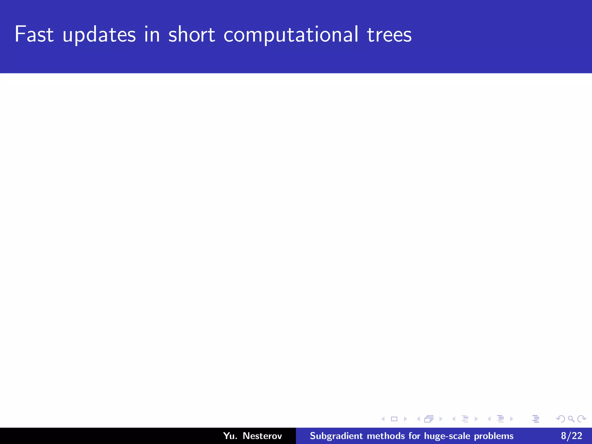
![When it can work?
Simple methods: No full-vector operations! (Is it possible?)
Simple problems: Functions with sparse gradients.
Let us try:
1 Quadratic function f (x) = 1
2 Ax, x − b, x . The gradient
f (x) = Ax − b, x ∈ RN
,
is not sparse even if A is sparse.
2 Piece-wise linear function g(x) = max
1≤i≤m
[ ai , x − b(i)]. Its
subgradient f (x) = ai(x), i(x) : f (x) = ai(x), x − b(i(x)),
can be sparse is ai is sparse!
Yu. Nesterov Subgradient methods for huge-scale problems 7/22](https://image.slidesharecdn.com/sublinbm1-141114054915-conversion-gate02/75/Subgradient-Methods-for-Huge-Scale-Optimization-Problems-Catholic-University-of-Louvain-Belgium-61-2048.jpg)
![When it can work?
Simple methods: No full-vector operations! (Is it possible?)
Simple problems: Functions with sparse gradients.
Let us try:
1 Quadratic function f (x) = 1
2 Ax, x − b, x . The gradient
f (x) = Ax − b, x ∈ RN
,
is not sparse even if A is sparse.
2 Piece-wise linear function g(x) = max
1≤i≤m
[ ai , x − b(i)]. Its
subgradient f (x) = ai(x), i(x) : f (x) = ai(x), x − b(i(x)),
can be sparse is ai is sparse!
But:
Yu. Nesterov Subgradient methods for huge-scale problems 7/22](https://image.slidesharecdn.com/sublinbm1-141114054915-conversion-gate02/75/Subgradient-Methods-for-Huge-Scale-Optimization-Problems-Catholic-University-of-Louvain-Belgium-62-2048.jpg)
![When it can work?
Simple methods: No full-vector operations! (Is it possible?)
Simple problems: Functions with sparse gradients.
Let us try:
1 Quadratic function f (x) = 1
2 Ax, x − b, x . The gradient
f (x) = Ax − b, x ∈ RN
,
is not sparse even if A is sparse.
2 Piece-wise linear function g(x) = max
1≤i≤m
[ ai , x − b(i)]. Its
subgradient f (x) = ai(x), i(x) : f (x) = ai(x), x − b(i(x)),
can be sparse is ai is sparse!
But: We need a fast procedure for updating max-type operations.
Yu. Nesterov Subgradient methods for huge-scale problems 7/22](https://image.slidesharecdn.com/sublinbm1-141114054915-conversion-gate02/75/Subgradient-Methods-for-Huge-Scale-Optimization-Problems-Catholic-University-of-Louvain-Belgium-63-2048.jpg)
![Main advantages
Important examples (symmetric functions)
f (x) = x p, p ≥ 1, ψi,j (t1, t2) ≡ [ |t1|p + |t2|p ]1/p
,
Yu. Nesterov Subgradient methods for huge-scale problems 9/22](https://image.slidesharecdn.com/sublinbm1-141114054915-conversion-gate02/75/Subgradient-Methods-for-Huge-Scale-Optimization-Problems-Catholic-University-of-Louvain-Belgium-71-2048.jpg)
![Main advantages
Important examples (symmetric functions)
f (x) = x p, p ≥ 1, ψi,j (t1, t2) ≡ [ |t1|p + |t2|p ]1/p
,
f (x) = ln
n
i=1
ex(i)
, ψi,j (t1, t2) ≡ ln (et1 + et2 ) ,
Yu. Nesterov Subgradient methods for huge-scale problems 9/22](https://image.slidesharecdn.com/sublinbm1-141114054915-conversion-gate02/75/Subgradient-Methods-for-Huge-Scale-Optimization-Problems-Catholic-University-of-Louvain-Belgium-72-2048.jpg)
![Main advantages
Important examples (symmetric functions)
f (x) = x p, p ≥ 1, ψi,j (t1, t2) ≡ [ |t1|p + |t2|p ]1/p
,
f (x) = ln
n
i=1
ex(i)
, ψi,j (t1, t2) ≡ ln (et1 + et2 ) ,
f (x) = max
1≤i≤n
x(i), ψi,j (t1, t2) ≡ max {t1, t2} .
Yu. Nesterov Subgradient methods for huge-scale problems 9/22](https://image.slidesharecdn.com/sublinbm1-141114054915-conversion-gate02/75/Subgradient-Methods-for-Huge-Scale-Optimization-Problems-Catholic-University-of-Louvain-Belgium-73-2048.jpg)
![Main advantages
Important examples (symmetric functions)
f (x) = x p, p ≥ 1, ψi,j (t1, t2) ≡ [ |t1|p + |t2|p ]1/p
,
f (x) = ln
n
i=1
ex(i)
, ψi,j (t1, t2) ≡ ln (et1 + et2 ) ,
f (x) = max
1≤i≤n
x(i), ψi,j (t1, t2) ≡ max {t1, t2} .
The binary tree requires only n − 1 auxiliary cells.
Yu. Nesterov Subgradient methods for huge-scale problems 9/22](https://image.slidesharecdn.com/sublinbm1-141114054915-conversion-gate02/75/Subgradient-Methods-for-Huge-Scale-Optimization-Problems-Catholic-University-of-Louvain-Belgium-74-2048.jpg)
![Main advantages
Important examples (symmetric functions)
f (x) = x p, p ≥ 1, ψi,j (t1, t2) ≡ [ |t1|p + |t2|p ]1/p
,
f (x) = ln
n
i=1
ex(i)
, ψi,j (t1, t2) ≡ ln (et1 + et2 ) ,
f (x) = max
1≤i≤n
x(i), ψi,j (t1, t2) ≡ max {t1, t2} .
The binary tree requires only n − 1 auxiliary cells.
Its value needs n − 1 applications of ψi,j (·, ·) ( ≡ operations).
Yu. Nesterov Subgradient methods for huge-scale problems 9/22](https://image.slidesharecdn.com/sublinbm1-141114054915-conversion-gate02/75/Subgradient-Methods-for-Huge-Scale-Optimization-Problems-Catholic-University-of-Louvain-Belgium-75-2048.jpg)
![Main advantages
Important examples (symmetric functions)
f (x) = x p, p ≥ 1, ψi,j (t1, t2) ≡ [ |t1|p + |t2|p ]1/p
,
f (x) = ln
n
i=1
ex(i)
, ψi,j (t1, t2) ≡ ln (et1 + et2 ) ,
f (x) = max
1≤i≤n
x(i), ψi,j (t1, t2) ≡ max {t1, t2} .
The binary tree requires only n − 1 auxiliary cells.
Its value needs n − 1 applications of ψi,j (·, ·) ( ≡ operations).
If x+ differs from x in one entry only, then for re-computing
f (x+) we need only k ≡ log2 n operations.
Yu. Nesterov Subgradient methods for huge-scale problems 9/22](https://image.slidesharecdn.com/sublinbm1-141114054915-conversion-gate02/75/Subgradient-Methods-for-Huge-Scale-Optimization-Problems-Catholic-University-of-Louvain-Belgium-76-2048.jpg)
![Main advantages
Important examples (symmetric functions)
f (x) = x p, p ≥ 1, ψi,j (t1, t2) ≡ [ |t1|p + |t2|p ]1/p
,
f (x) = ln
n
i=1
ex(i)
, ψi,j (t1, t2) ≡ ln (et1 + et2 ) ,
f (x) = max
1≤i≤n
x(i), ψi,j (t1, t2) ≡ max {t1, t2} .
The binary tree requires only n − 1 auxiliary cells.
Its value needs n − 1 applications of ψi,j (·, ·) ( ≡ operations).
If x+ differs from x in one entry only, then for re-computing
f (x+) we need only k ≡ log2 n operations.
Thus, we can have pure subgradient minimization schemes with
Yu. Nesterov Subgradient methods for huge-scale problems 9/22](https://image.slidesharecdn.com/sublinbm1-141114054915-conversion-gate02/75/Subgradient-Methods-for-Huge-Scale-Optimization-Problems-Catholic-University-of-Louvain-Belgium-77-2048.jpg)
![Main advantages
Important examples (symmetric functions)
f (x) = x p, p ≥ 1, ψi,j (t1, t2) ≡ [ |t1|p + |t2|p ]1/p
,
f (x) = ln
n
i=1
ex(i)
, ψi,j (t1, t2) ≡ ln (et1 + et2 ) ,
f (x) = max
1≤i≤n
x(i), ψi,j (t1, t2) ≡ max {t1, t2} .
The binary tree requires only n − 1 auxiliary cells.
Its value needs n − 1 applications of ψi,j (·, ·) ( ≡ operations).
If x+ differs from x in one entry only, then for re-computing
f (x+) we need only k ≡ log2 n operations.
Thus, we can have pure subgradient minimization schemes with
Sublinear Iteration Cost
.
Yu. Nesterov Subgradient methods for huge-scale problems 9/22](https://image.slidesharecdn.com/sublinbm1-141114054915-conversion-gate02/75/Subgradient-Methods-for-Huge-Scale-Optimization-Problems-Catholic-University-of-Louvain-Belgium-78-2048.jpg)


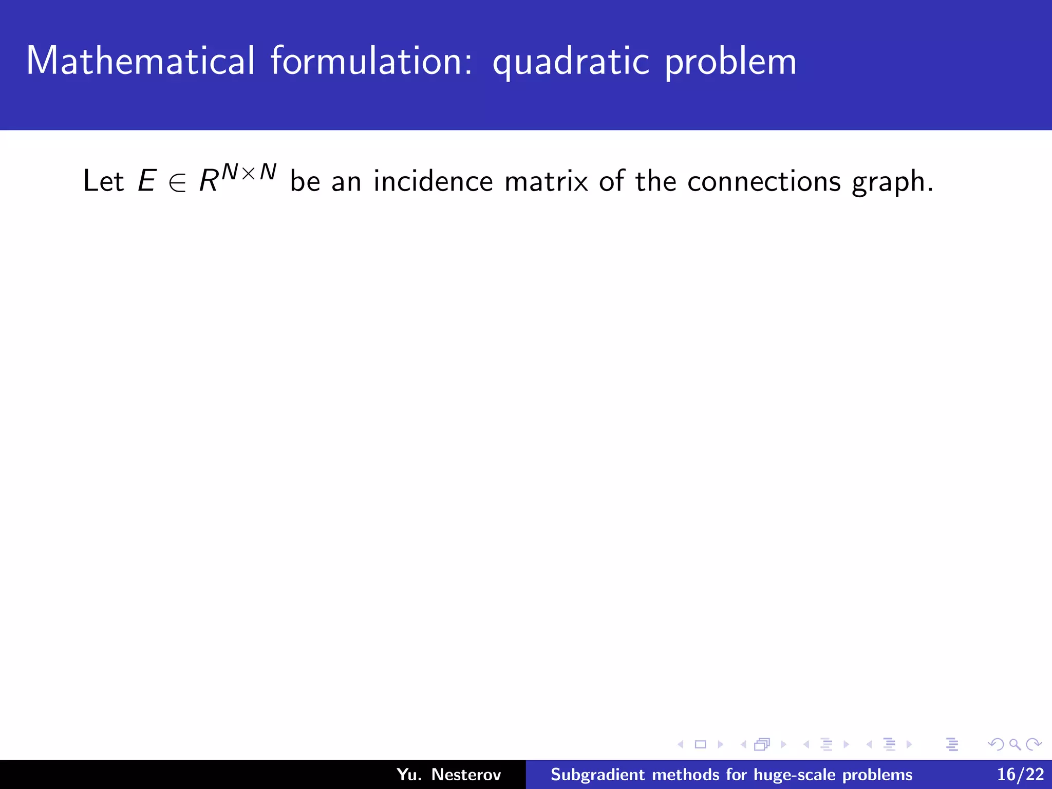
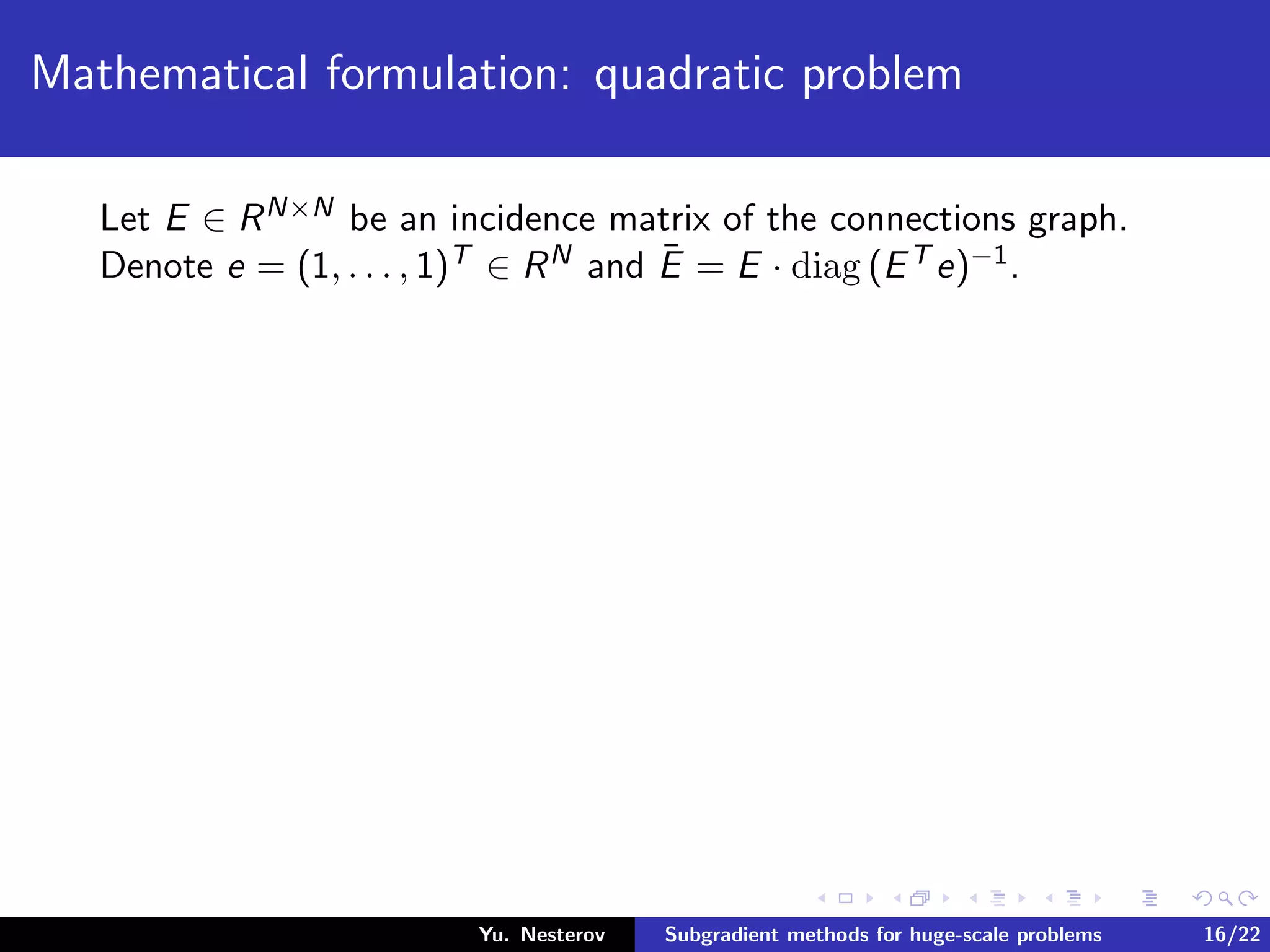
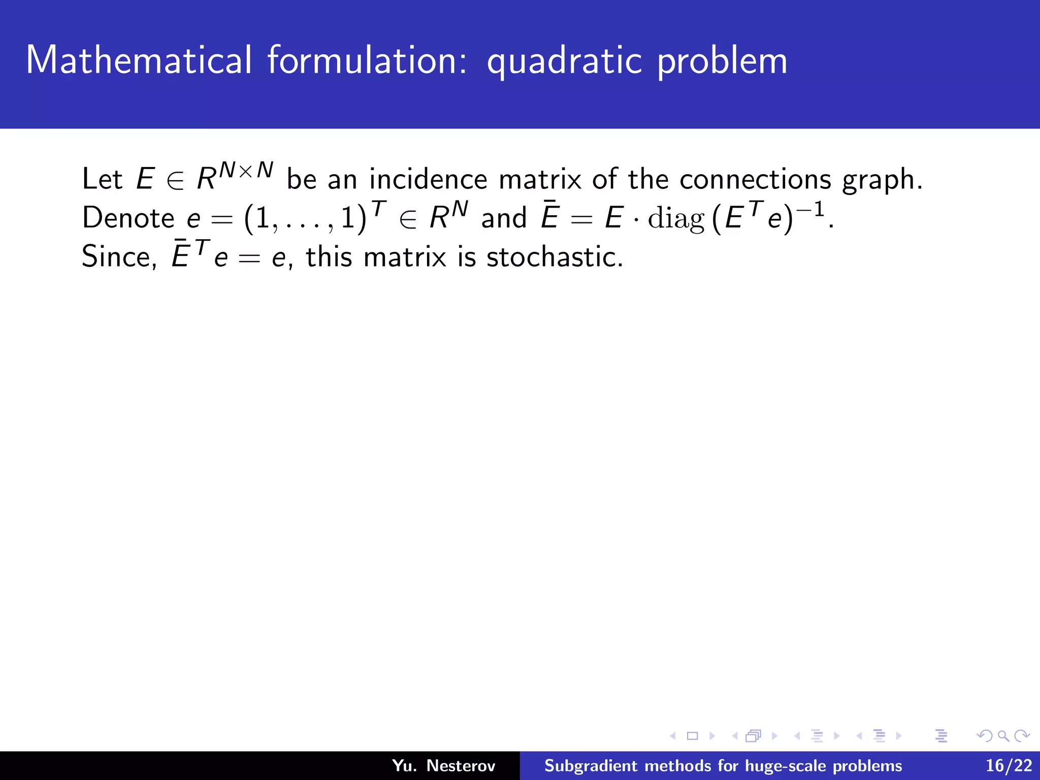
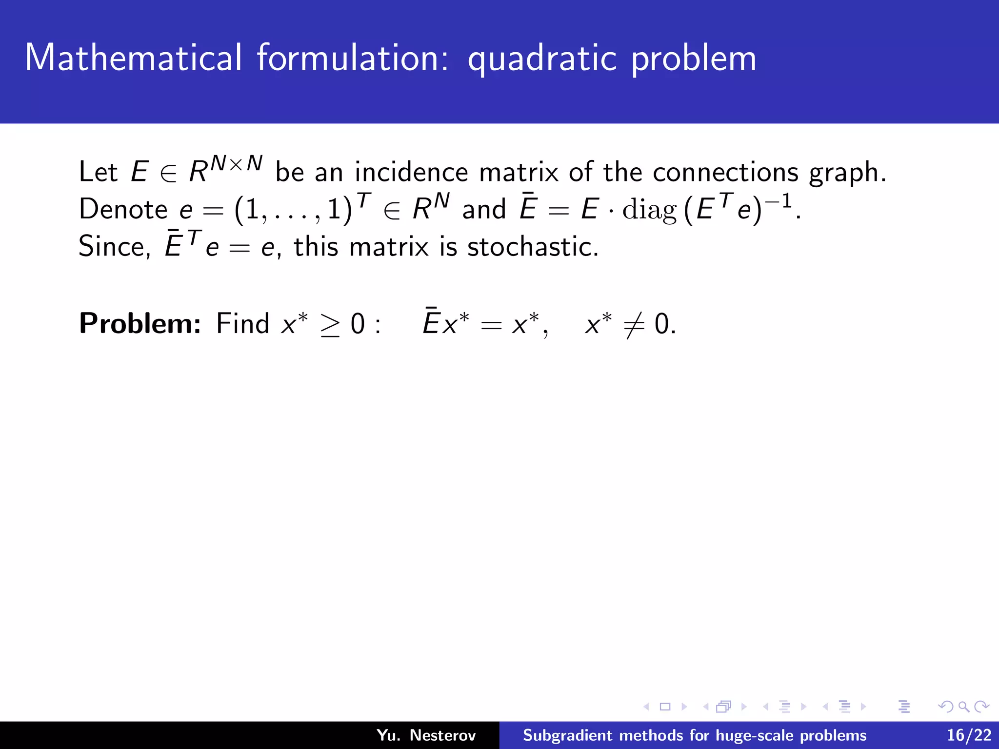
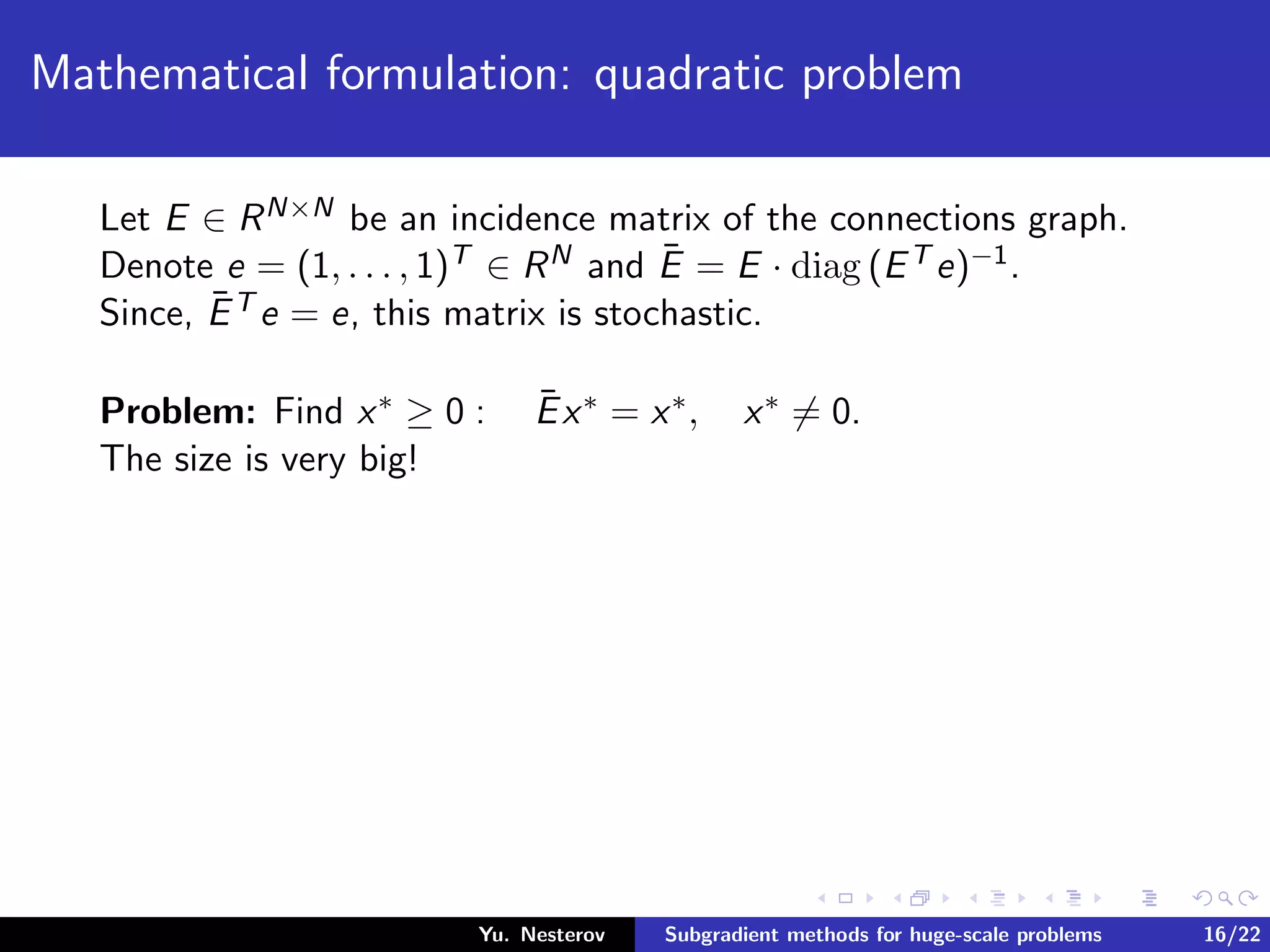
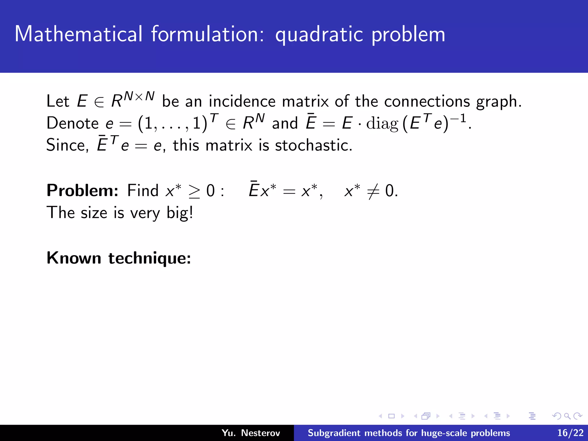
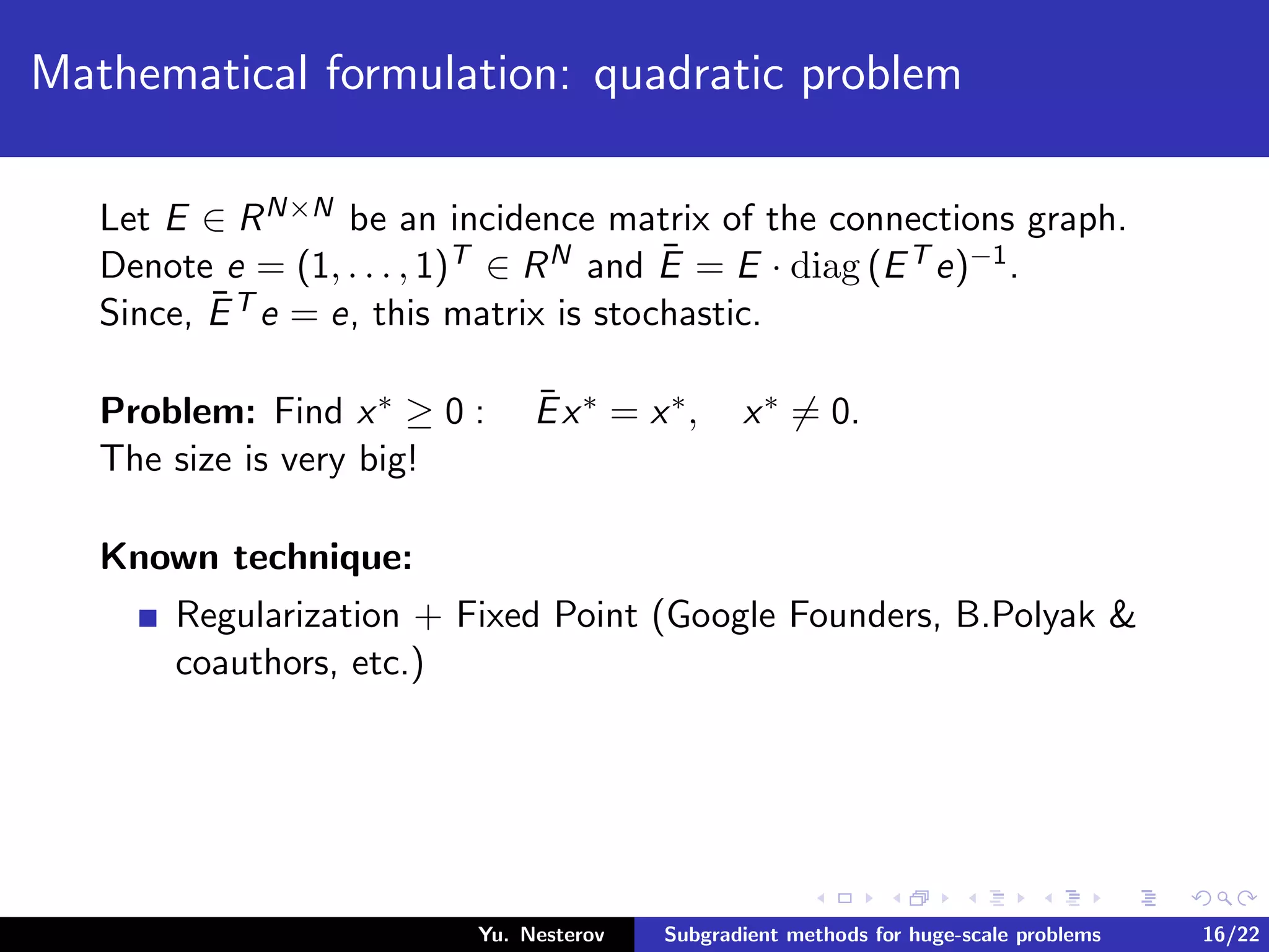
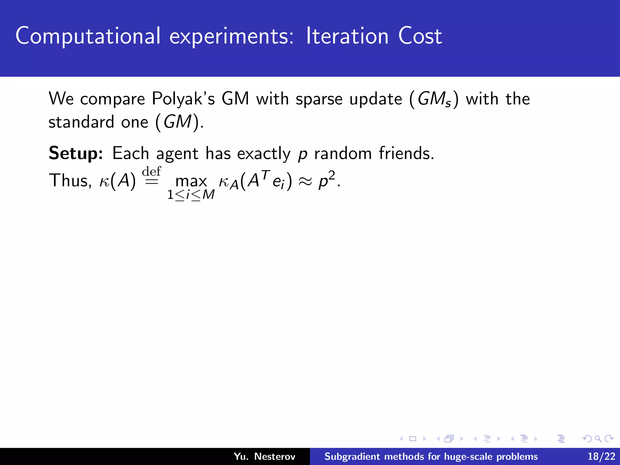
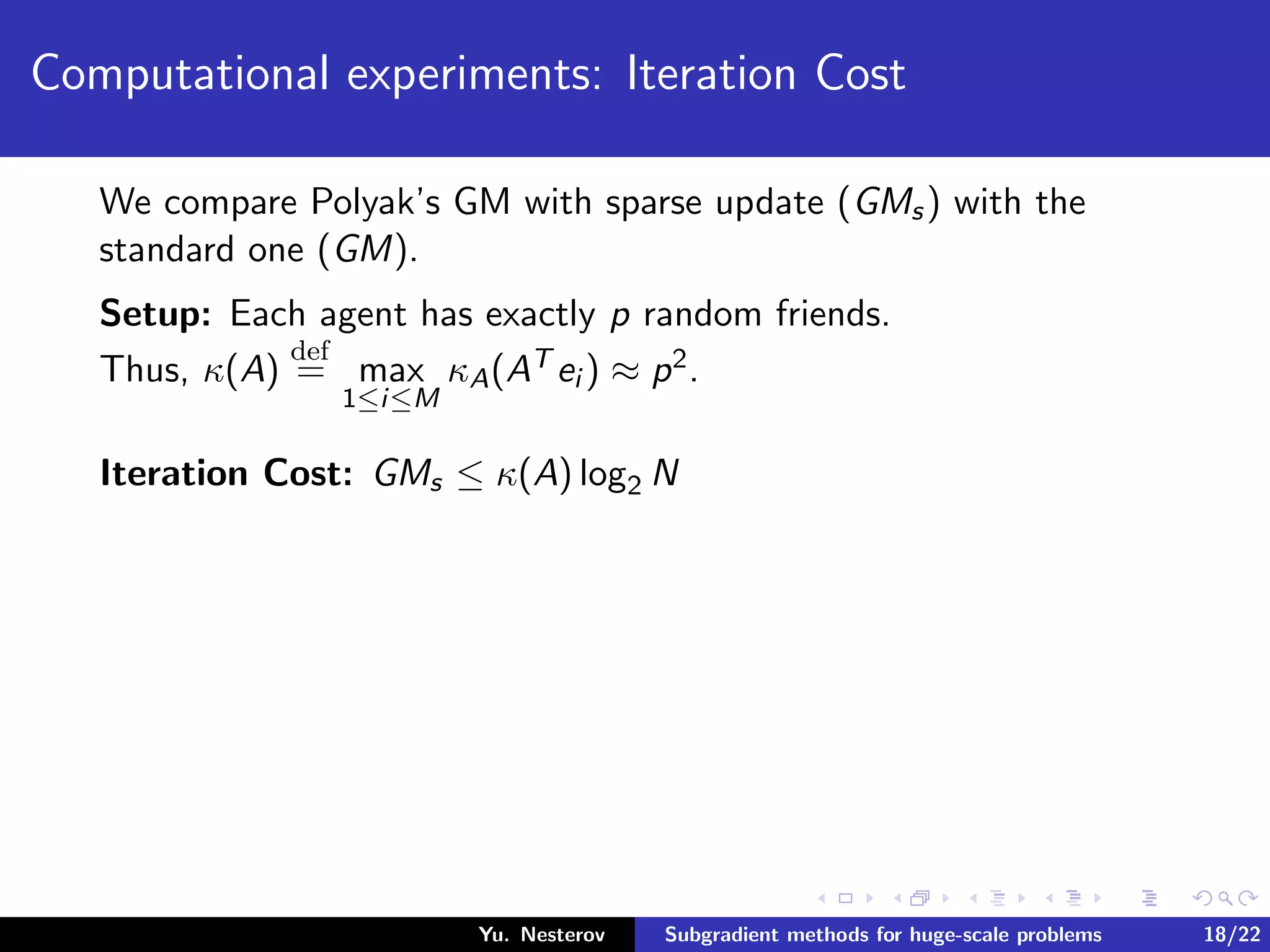
![Mathematical formulation: quadratic problem
Let E ∈ RN×N be an incidence matrix of the connections graph.
Denote e = (1, . . . , 1)T ∈ RN and ¯E = E · diag (ET e)−1.
Since, ¯ET e = e, this matrix is stochastic.
Problem: Find x∗ ≥ 0 : ¯Ex∗ = x∗, x∗ = 0.
The size is very big!
Known technique:
Regularization + Fixed Point (Google Founders, B.Polyak &
coauthors, etc.)
N09: Solve it by random CD-method as applied to
1
2
¯Ex − x 2 + γ
2 [ e, x − 1]2, γ > 0.
Yu. Nesterov Subgradient methods for huge-scale problems 16/22](https://image.slidesharecdn.com/sublinbm1-141114054915-conversion-gate02/75/Subgradient-Methods-for-Huge-Scale-Optimization-Problems-Catholic-University-of-Louvain-Belgium-151-2048.jpg)
![Mathematical formulation: quadratic problem
Let E ∈ RN×N be an incidence matrix of the connections graph.
Denote e = (1, . . . , 1)T ∈ RN and ¯E = E · diag (ET e)−1.
Since, ¯ET e = e, this matrix is stochastic.
Problem: Find x∗ ≥ 0 : ¯Ex∗ = x∗, x∗ = 0.
The size is very big!
Known technique:
Regularization + Fixed Point (Google Founders, B.Polyak &
coauthors, etc.)
N09: Solve it by random CD-method as applied to
1
2
¯Ex − x 2 + γ
2 [ e, x − 1]2, γ > 0.
Main drawback: No interpretation for the objective function!
Yu. Nesterov Subgradient methods for huge-scale problems 16/22](https://image.slidesharecdn.com/sublinbm1-141114054915-conversion-gate02/75/Subgradient-Methods-for-Huge-Scale-Optimization-Problems-Catholic-University-of-Louvain-Belgium-152-2048.jpg)
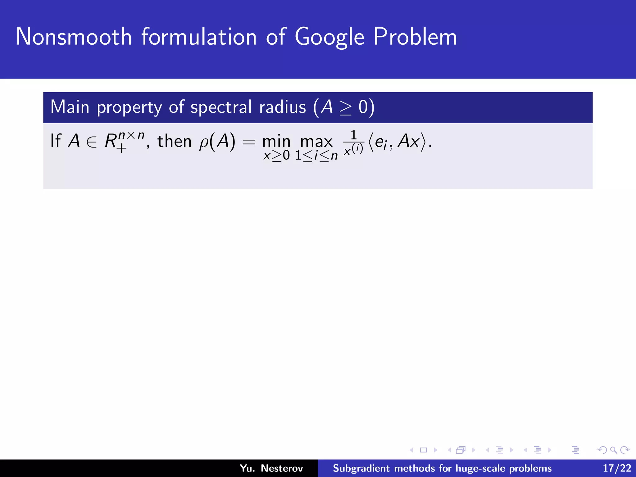
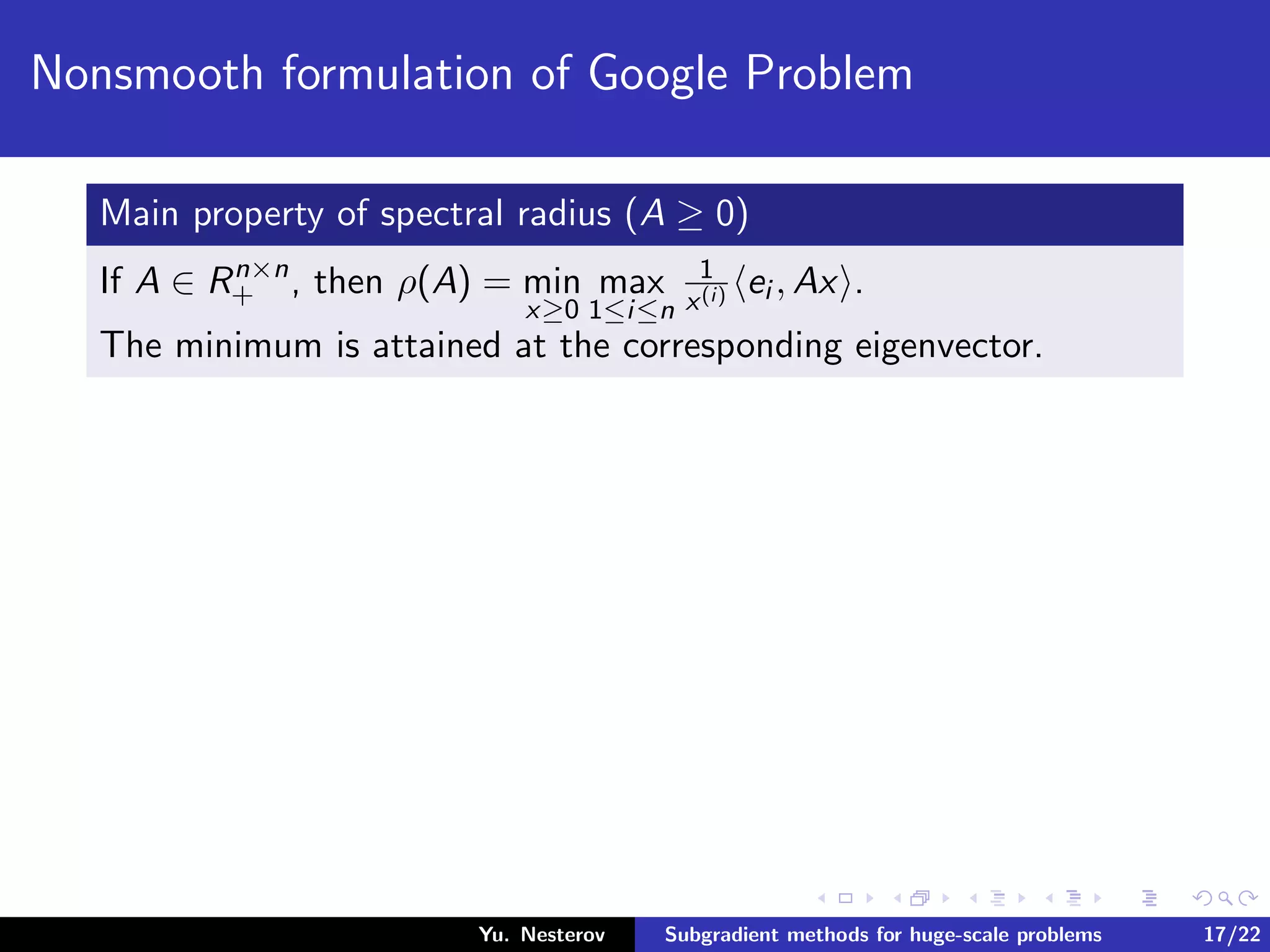
![Nonsmooth formulation of Google Problem
Main property of spectral radius (A ≥ 0)
If A ∈ Rn×n
+ , then ρ(A) = min
x≥0
max
1≤i≤n
1
x(i) ei , Ax .
The minimum is attained at the corresponding eigenvector.
Since ρ(¯E) = 1, our problem is as follows:
f (x)
def
= max
1≤i≤N
[ ei , ¯Ex − x(i)] → min
x≥0
.
Yu. Nesterov Subgradient methods for huge-scale problems 17/22](https://image.slidesharecdn.com/sublinbm1-141114054915-conversion-gate02/75/Subgradient-Methods-for-Huge-Scale-Optimization-Problems-Catholic-University-of-Louvain-Belgium-156-2048.jpg)
![Nonsmooth formulation of Google Problem
Main property of spectral radius (A ≥ 0)
If A ∈ Rn×n
+ , then ρ(A) = min
x≥0
max
1≤i≤n
1
x(i) ei , Ax .
The minimum is attained at the corresponding eigenvector.
Since ρ(¯E) = 1, our problem is as follows:
f (x)
def
= max
1≤i≤N
[ ei , ¯Ex − x(i)] → min
x≥0
.
Interpretation: Increase self-confidence!
Yu. Nesterov Subgradient methods for huge-scale problems 17/22](https://image.slidesharecdn.com/sublinbm1-141114054915-conversion-gate02/75/Subgradient-Methods-for-Huge-Scale-Optimization-Problems-Catholic-University-of-Louvain-Belgium-157-2048.jpg)
![Nonsmooth formulation of Google Problem
Main property of spectral radius (A ≥ 0)
If A ∈ Rn×n
+ , then ρ(A) = min
x≥0
max
1≤i≤n
1
x(i) ei , Ax .
The minimum is attained at the corresponding eigenvector.
Since ρ(¯E) = 1, our problem is as follows:
f (x)
def
= max
1≤i≤N
[ ei , ¯Ex − x(i)] → min
x≥0
.
Interpretation: Increase self-confidence!
Since f ∗ = 0, we can apply Polyak’s method with sparse updates.
Yu. Nesterov Subgradient methods for huge-scale problems 17/22](https://image.slidesharecdn.com/sublinbm1-141114054915-conversion-gate02/75/Subgradient-Methods-for-Huge-Scale-Optimization-Problems-Catholic-University-of-Louvain-Belgium-158-2048.jpg)
![Nonsmooth formulation of Google Problem
Main property of spectral radius (A ≥ 0)
If A ∈ Rn×n
+ , then ρ(A) = min
x≥0
max
1≤i≤n
1
x(i) ei , Ax .
The minimum is attained at the corresponding eigenvector.
Since ρ(¯E) = 1, our problem is as follows:
f (x)
def
= max
1≤i≤N
[ ei , ¯Ex − x(i)] → min
x≥0
.
Interpretation: Increase self-confidence!
Since f ∗ = 0, we can apply Polyak’s method with sparse updates.
Additional features; the optimal set X∗ is a convex cone.
Yu. Nesterov Subgradient methods for huge-scale problems 17/22](https://image.slidesharecdn.com/sublinbm1-141114054915-conversion-gate02/75/Subgradient-Methods-for-Huge-Scale-Optimization-Problems-Catholic-University-of-Louvain-Belgium-159-2048.jpg)
![Nonsmooth formulation of Google Problem
Main property of spectral radius (A ≥ 0)
If A ∈ Rn×n
+ , then ρ(A) = min
x≥0
max
1≤i≤n
1
x(i) ei , Ax .
The minimum is attained at the corresponding eigenvector.
Since ρ(¯E) = 1, our problem is as follows:
f (x)
def
= max
1≤i≤N
[ ei , ¯Ex − x(i)] → min
x≥0
.
Interpretation: Increase self-confidence!
Since f ∗ = 0, we can apply Polyak’s method with sparse updates.
Additional features; the optimal set X∗ is a convex cone.
If x0 = e, then the whole sequence is separated from zero:
Yu. Nesterov Subgradient methods for huge-scale problems 17/22](https://image.slidesharecdn.com/sublinbm1-141114054915-conversion-gate02/75/Subgradient-Methods-for-Huge-Scale-Optimization-Problems-Catholic-University-of-Louvain-Belgium-160-2048.jpg)
![Nonsmooth formulation of Google Problem
Main property of spectral radius (A ≥ 0)
If A ∈ Rn×n
+ , then ρ(A) = min
x≥0
max
1≤i≤n
1
x(i) ei , Ax .
The minimum is attained at the corresponding eigenvector.
Since ρ(¯E) = 1, our problem is as follows:
f (x)
def
= max
1≤i≤N
[ ei , ¯Ex − x(i)] → min
x≥0
.
Interpretation: Increase self-confidence!
Since f ∗ = 0, we can apply Polyak’s method with sparse updates.
Additional features; the optimal set X∗ is a convex cone.
If x0 = e, then the whole sequence is separated from zero:
x∗, e
Yu. Nesterov Subgradient methods for huge-scale problems 17/22](https://image.slidesharecdn.com/sublinbm1-141114054915-conversion-gate02/75/Subgradient-Methods-for-Huge-Scale-Optimization-Problems-Catholic-University-of-Louvain-Belgium-161-2048.jpg)
![Nonsmooth formulation of Google Problem
Main property of spectral radius (A ≥ 0)
If A ∈ Rn×n
+ , then ρ(A) = min
x≥0
max
1≤i≤n
1
x(i) ei , Ax .
The minimum is attained at the corresponding eigenvector.
Since ρ(¯E) = 1, our problem is as follows:
f (x)
def
= max
1≤i≤N
[ ei , ¯Ex − x(i)] → min
x≥0
.
Interpretation: Increase self-confidence!
Since f ∗ = 0, we can apply Polyak’s method with sparse updates.
Additional features; the optimal set X∗ is a convex cone.
If x0 = e, then the whole sequence is separated from zero:
x∗, e ≤ x∗, xk
Yu. Nesterov Subgradient methods for huge-scale problems 17/22](https://image.slidesharecdn.com/sublinbm1-141114054915-conversion-gate02/75/Subgradient-Methods-for-Huge-Scale-Optimization-Problems-Catholic-University-of-Louvain-Belgium-162-2048.jpg)
![Nonsmooth formulation of Google Problem
Main property of spectral radius (A ≥ 0)
If A ∈ Rn×n
+ , then ρ(A) = min
x≥0
max
1≤i≤n
1
x(i) ei , Ax .
The minimum is attained at the corresponding eigenvector.
Since ρ(¯E) = 1, our problem is as follows:
f (x)
def
= max
1≤i≤N
[ ei , ¯Ex − x(i)] → min
x≥0
.
Interpretation: Increase self-confidence!
Since f ∗ = 0, we can apply Polyak’s method with sparse updates.
Additional features; the optimal set X∗ is a convex cone.
If x0 = e, then the whole sequence is separated from zero:
x∗, e ≤ x∗, xk ≤ x∗
1 · xk ∞
Yu. Nesterov Subgradient methods for huge-scale problems 17/22](https://image.slidesharecdn.com/sublinbm1-141114054915-conversion-gate02/75/Subgradient-Methods-for-Huge-Scale-Optimization-Problems-Catholic-University-of-Louvain-Belgium-163-2048.jpg)
![Nonsmooth formulation of Google Problem
Main property of spectral radius (A ≥ 0)
If A ∈ Rn×n
+ , then ρ(A) = min
x≥0
max
1≤i≤n
1
x(i) ei , Ax .
The minimum is attained at the corresponding eigenvector.
Since ρ(¯E) = 1, our problem is as follows:
f (x)
def
= max
1≤i≤N
[ ei , ¯Ex − x(i)] → min
x≥0
.
Interpretation: Increase self-confidence!
Since f ∗ = 0, we can apply Polyak’s method with sparse updates.
Additional features; the optimal set X∗ is a convex cone.
If x0 = e, then the whole sequence is separated from zero:
x∗, e ≤ x∗, xk ≤ x∗
1 · xk ∞ = x∗, e · xk ∞.
Yu. Nesterov Subgradient methods for huge-scale problems 17/22](https://image.slidesharecdn.com/sublinbm1-141114054915-conversion-gate02/75/Subgradient-Methods-for-Huge-Scale-Optimization-Problems-Catholic-University-of-Louvain-Belgium-164-2048.jpg)
![Nonsmooth formulation of Google Problem
Main property of spectral radius (A ≥ 0)
If A ∈ Rn×n
+ , then ρ(A) = min
x≥0
max
1≤i≤n
1
x(i) ei , Ax .
The minimum is attained at the corresponding eigenvector.
Since ρ(¯E) = 1, our problem is as follows:
f (x)
def
= max
1≤i≤N
[ ei , ¯Ex − x(i)] → min
x≥0
.
Interpretation: Increase self-confidence!
Since f ∗ = 0, we can apply Polyak’s method with sparse updates.
Additional features; the optimal set X∗ is a convex cone.
If x0 = e, then the whole sequence is separated from zero:
x∗, e ≤ x∗, xk ≤ x∗
1 · xk ∞ = x∗, e · xk ∞.
Goal: Find ¯x ≥ 0 such that ¯x ∞ ≥ 1 and f (¯x) ≤ .
Yu. Nesterov Subgradient methods for huge-scale problems 17/22](https://image.slidesharecdn.com/sublinbm1-141114054915-conversion-gate02/75/Subgradient-Methods-for-Huge-Scale-Optimization-Problems-Catholic-University-of-Louvain-Belgium-165-2048.jpg)
![Nonsmooth formulation of Google Problem
Main property of spectral radius (A ≥ 0)
If A ∈ Rn×n
+ , then ρ(A) = min
x≥0
max
1≤i≤n
1
x(i) ei , Ax .
The minimum is attained at the corresponding eigenvector.
Since ρ(¯E) = 1, our problem is as follows:
f (x)
def
= max
1≤i≤N
[ ei , ¯Ex − x(i)] → min
x≥0
.
Interpretation: Increase self-confidence!
Since f ∗ = 0, we can apply Polyak’s method with sparse updates.
Additional features; the optimal set X∗ is a convex cone.
If x0 = e, then the whole sequence is separated from zero:
x∗, e ≤ x∗, xk ≤ x∗
1 · xk ∞ = x∗, e · xk ∞.
Goal: Find ¯x ≥ 0 such that ¯x ∞ ≥ 1 and f (¯x) ≤ .
(First condition is satisfied automatically.)
Yu. Nesterov Subgradient methods for huge-scale problems 17/22](https://image.slidesharecdn.com/sublinbm1-141114054915-conversion-gate02/75/Subgradient-Methods-for-Huge-Scale-Optimization-Problems-Catholic-University-of-Louvain-Belgium-166-2048.jpg)

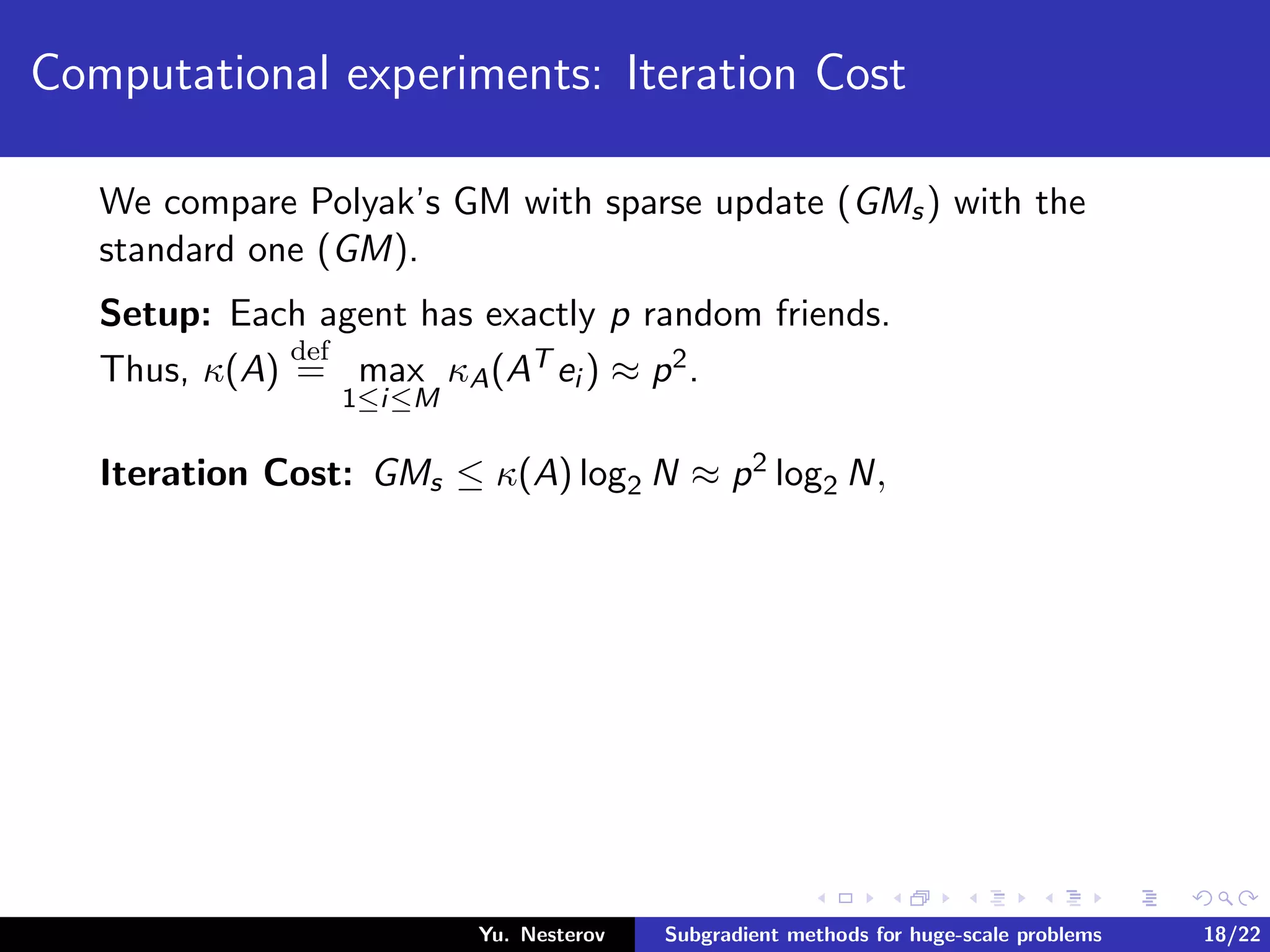
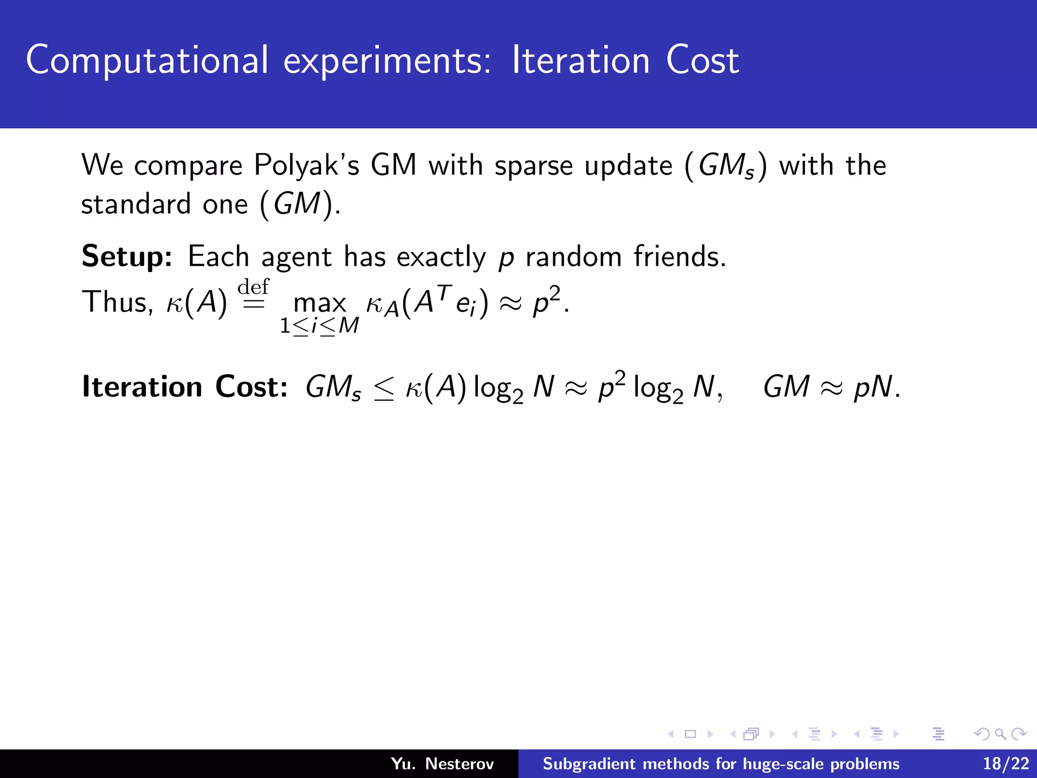
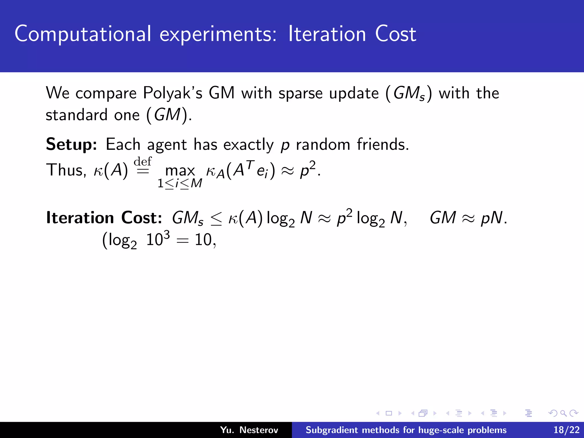
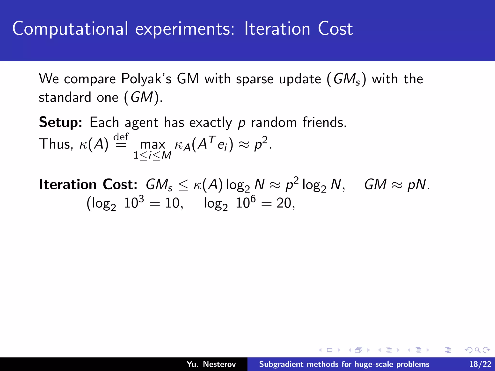
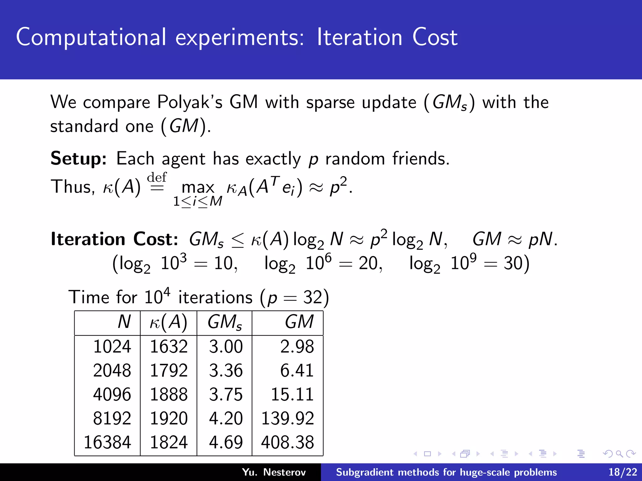

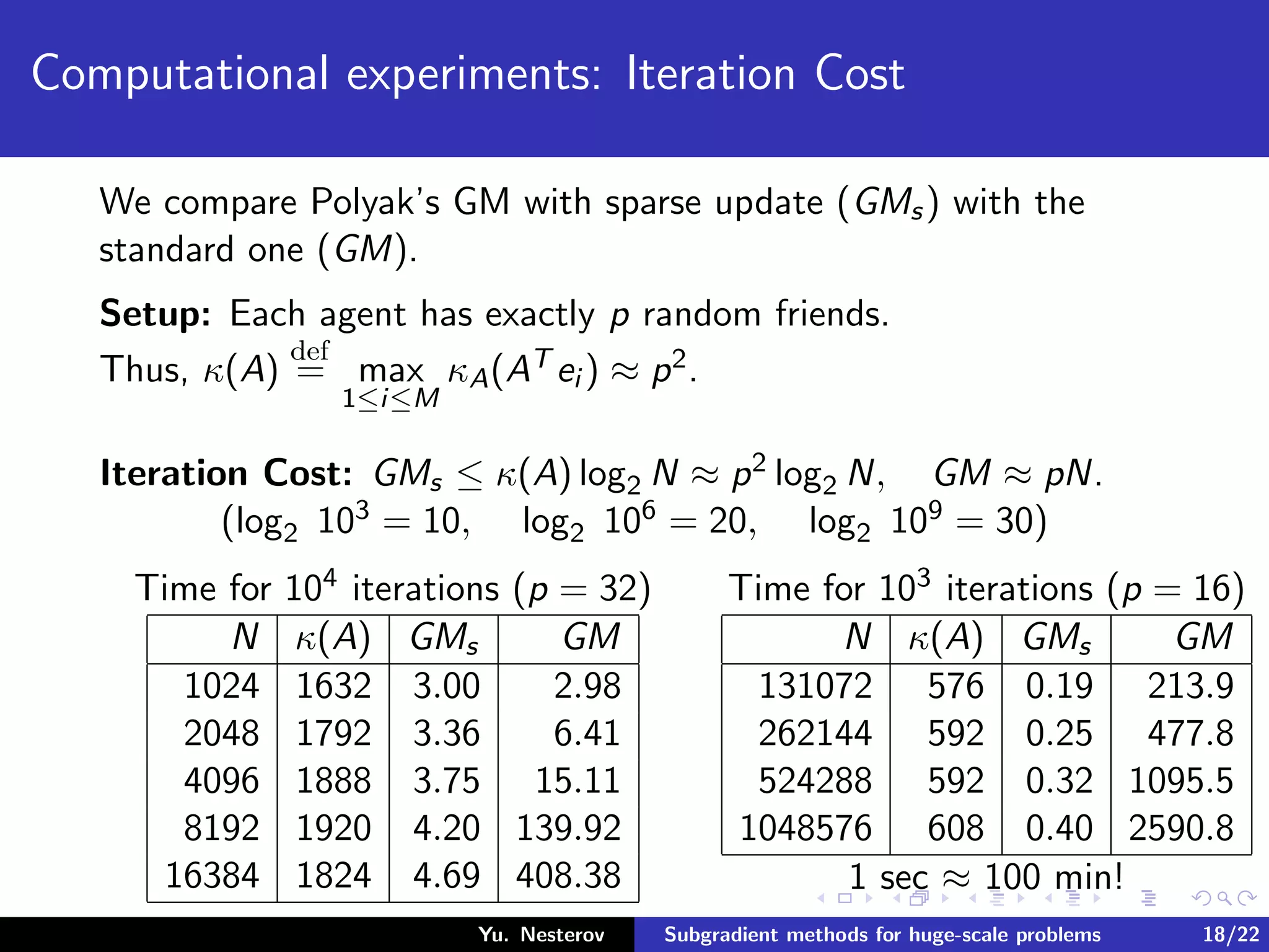
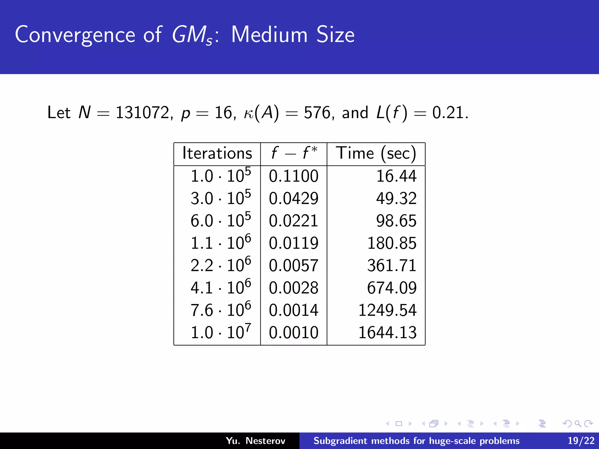
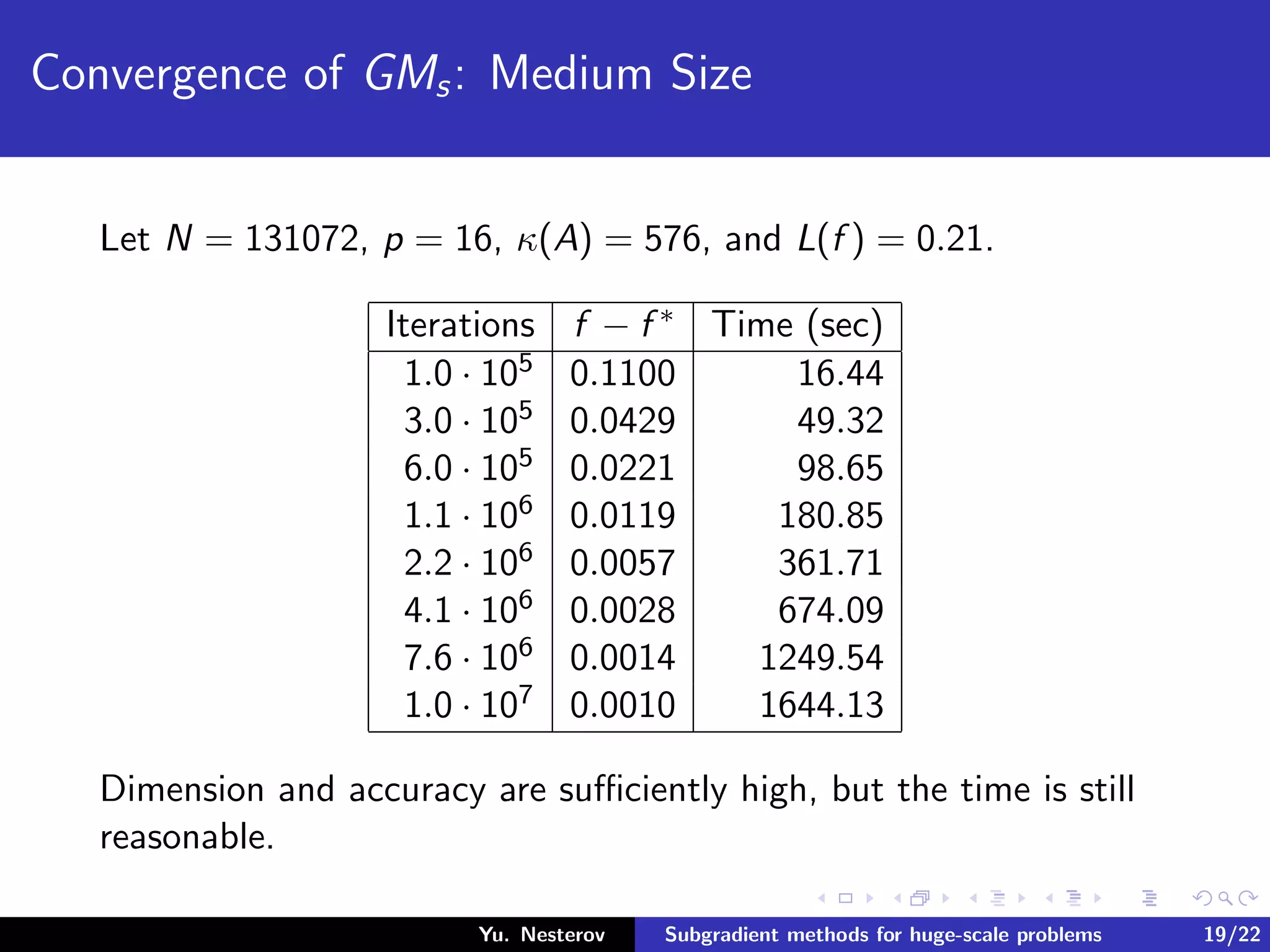


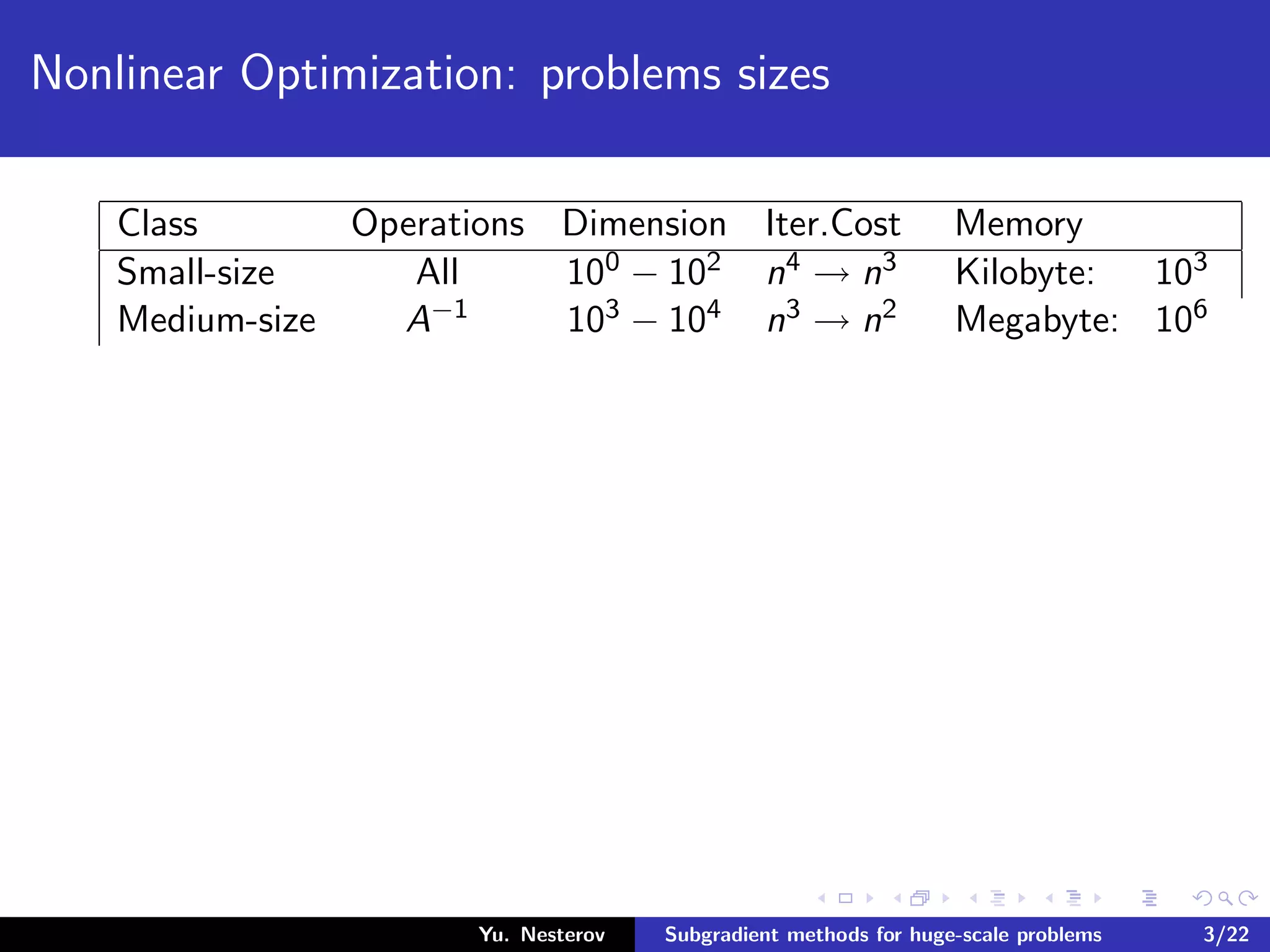
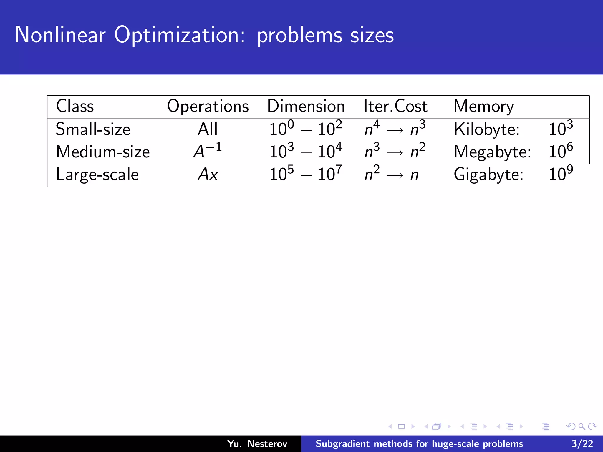
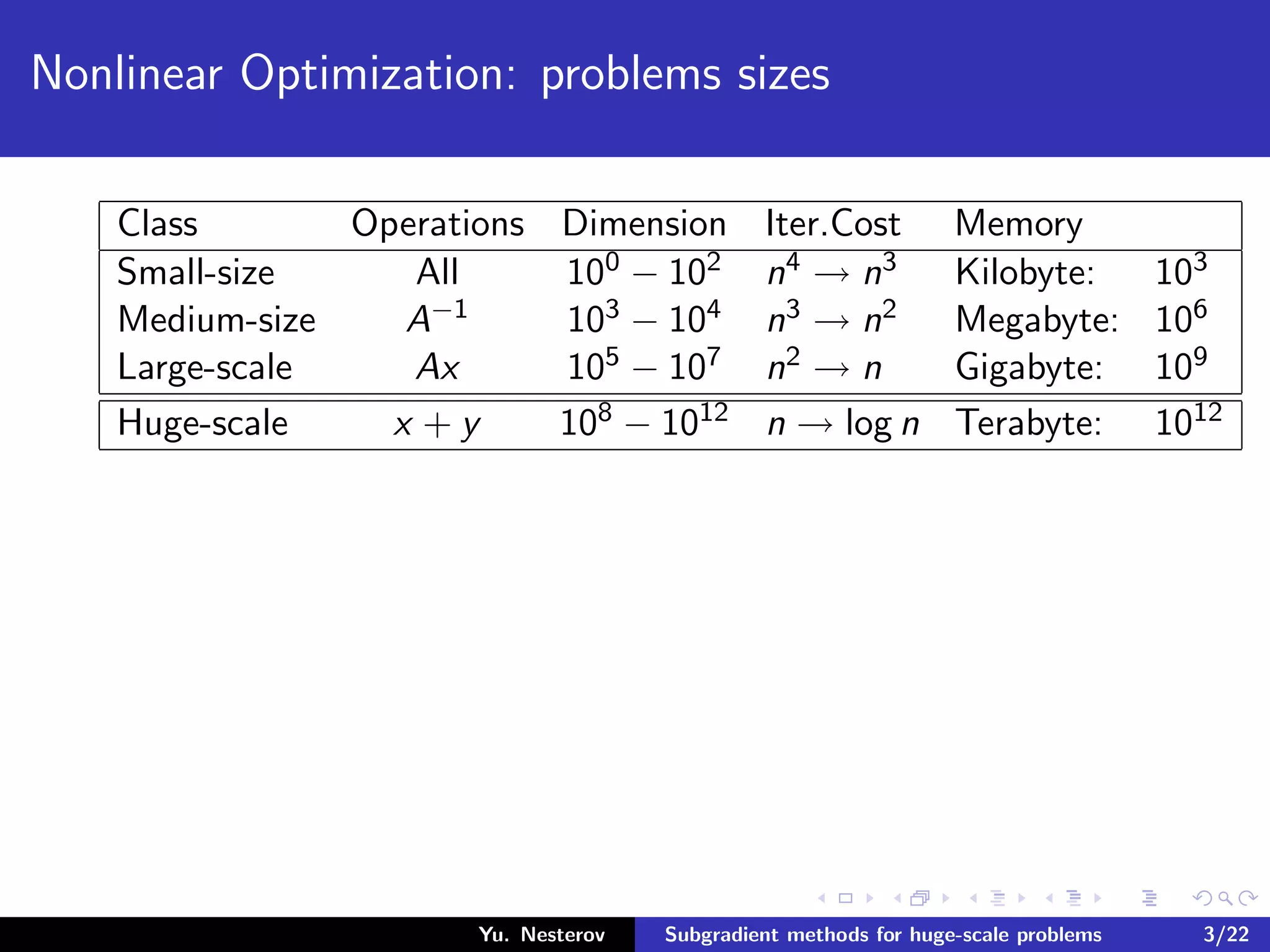
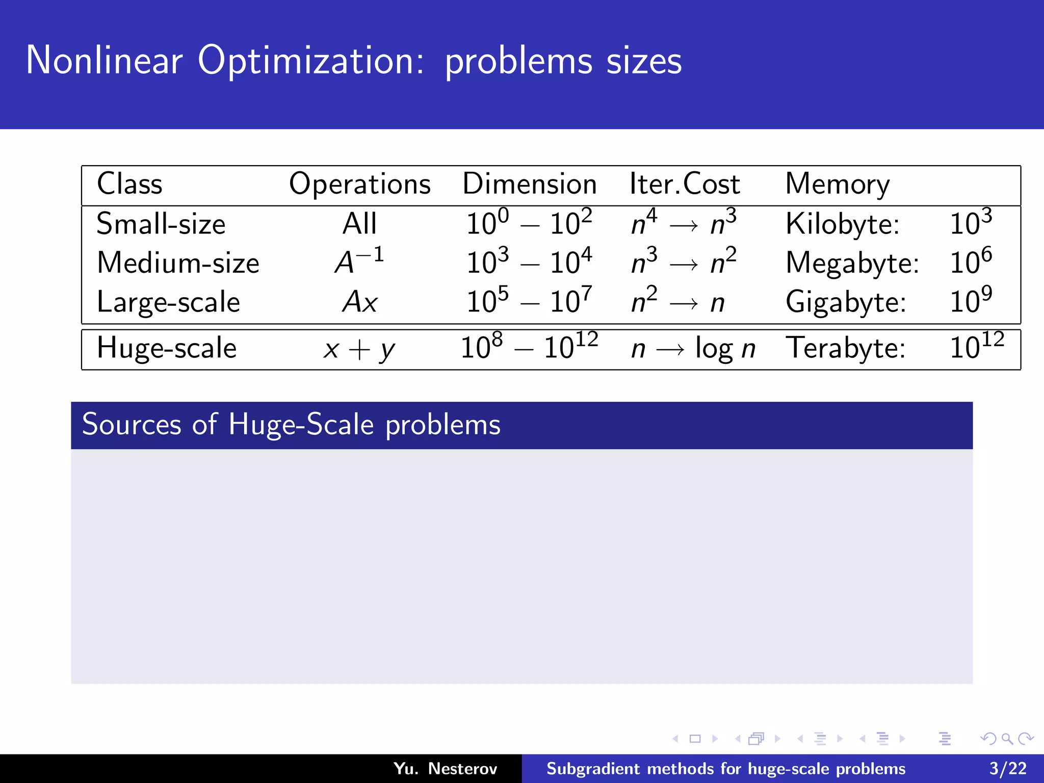
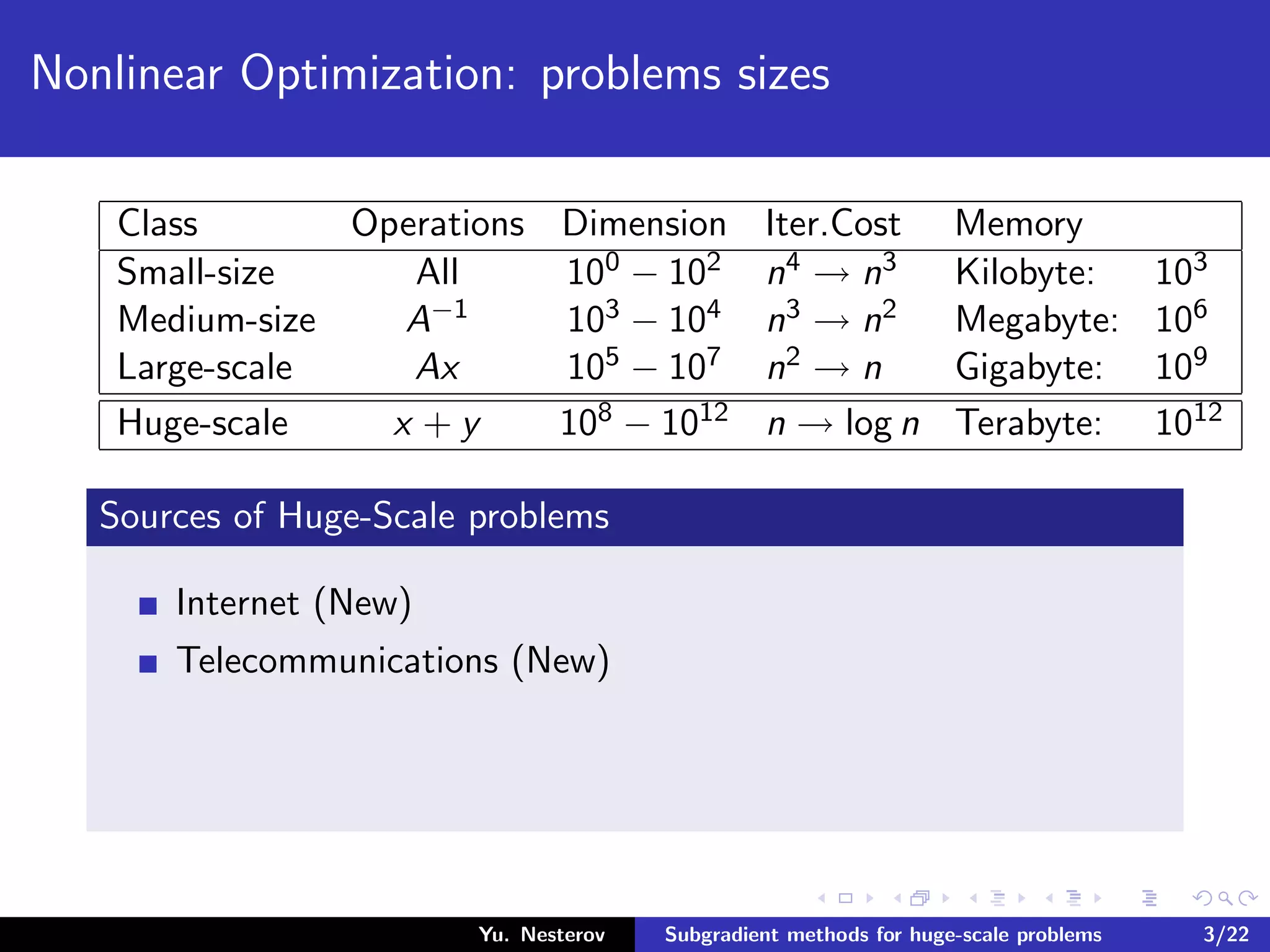
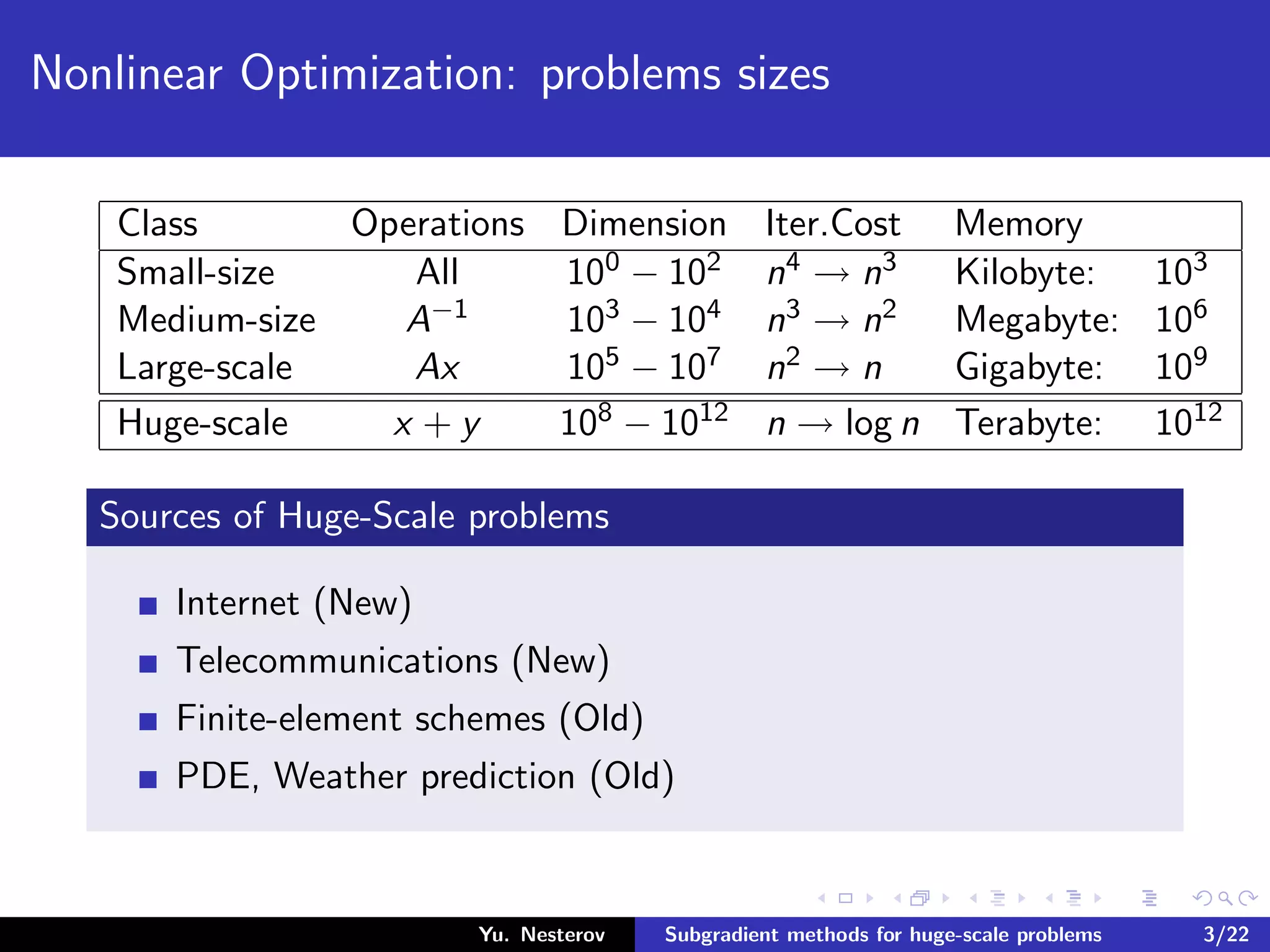
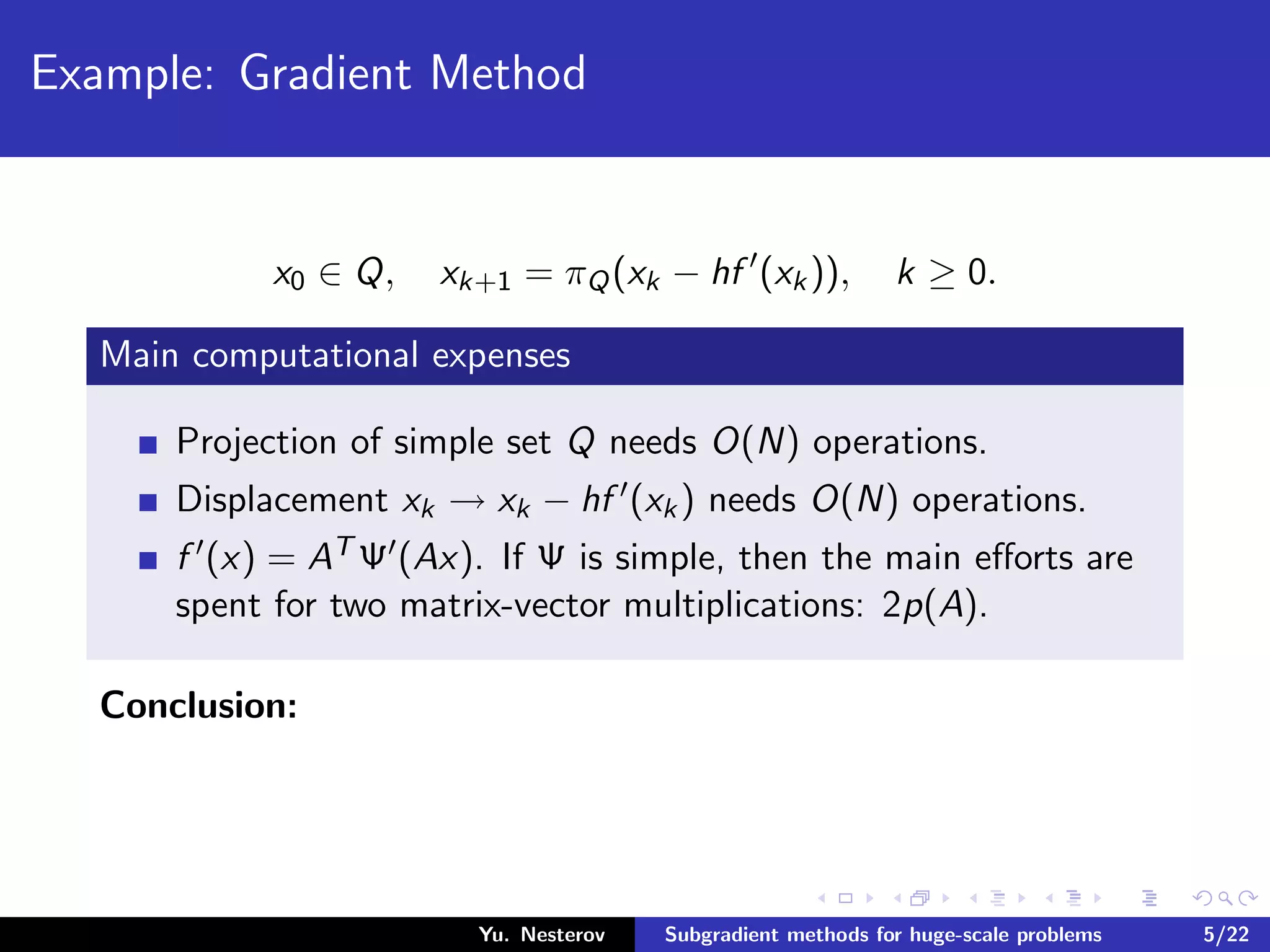
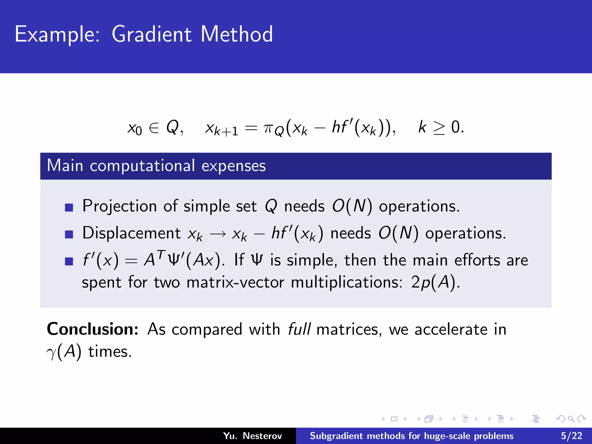
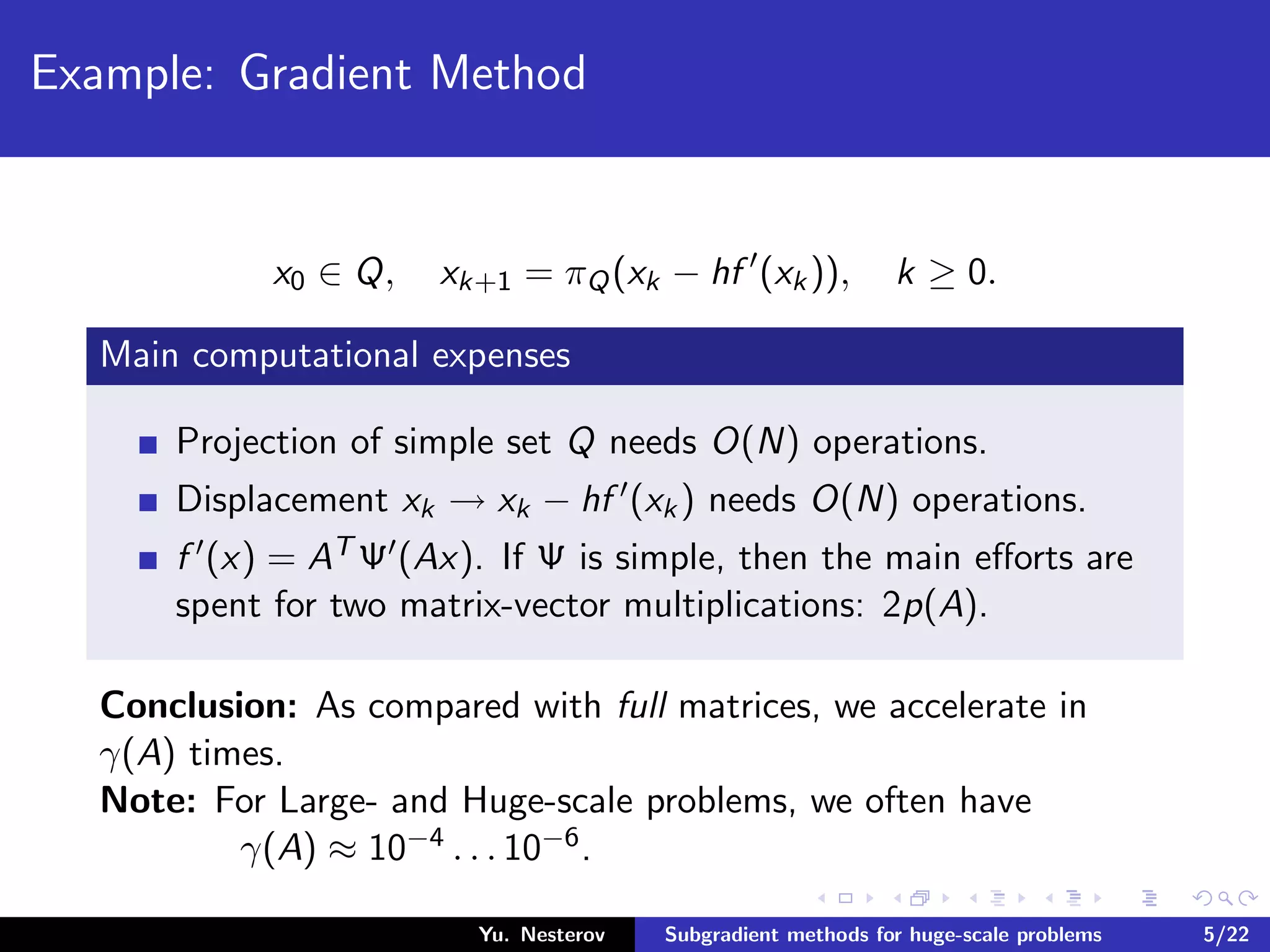
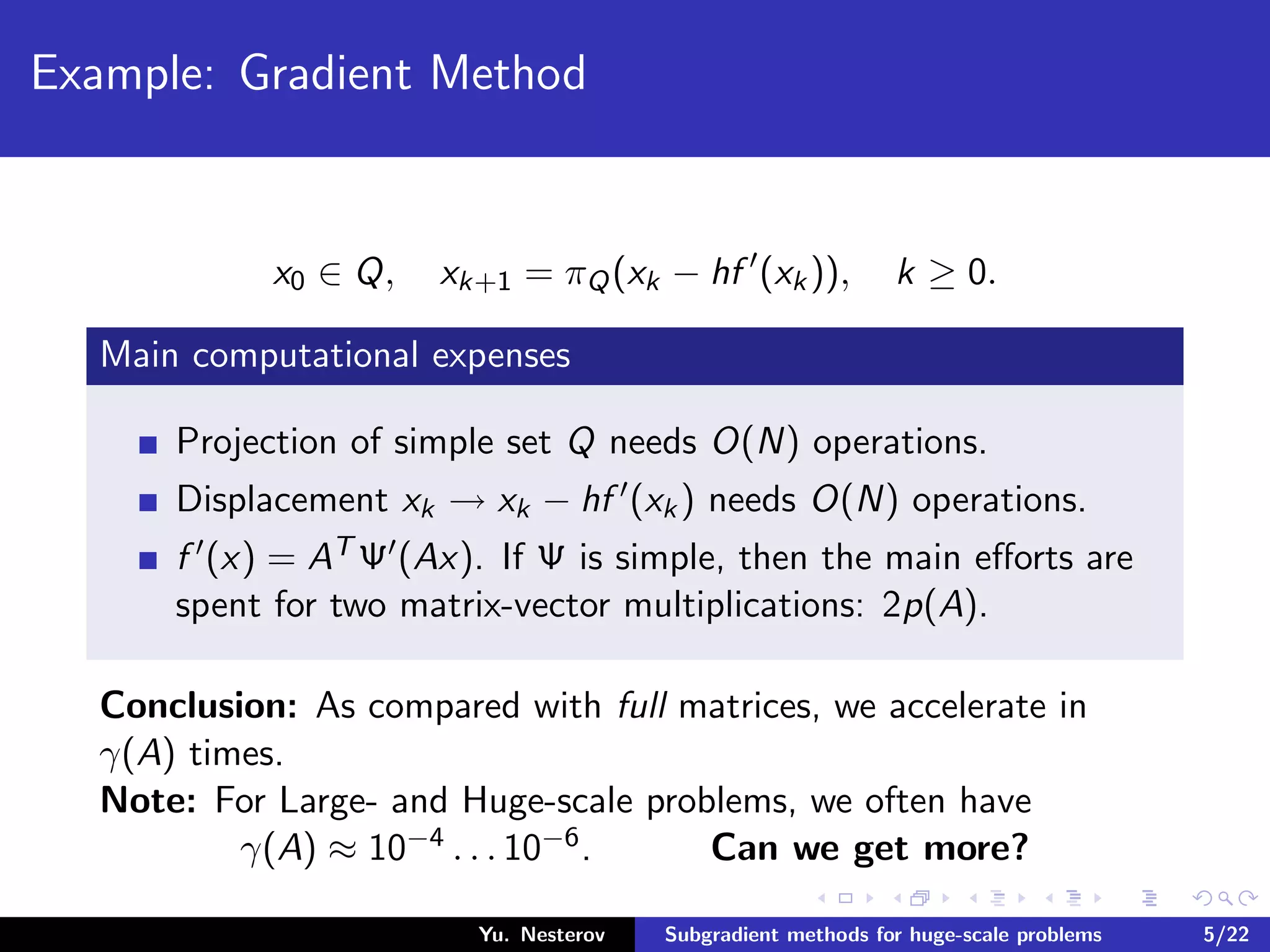
The document discusses subgradient methods for huge-scale optimization problems, highlighting the challenges and complexities involved in sparse optimization. It emphasizes the importance of sparsity in accelerating computations and provides examples of computational expenses for various algorithms. The author outlines strategies for sparse updates which significantly reduce the computational burden in comparison to traditional methods.


![Number_Guessing_Game_Dsbsbssbzboc[1].pptx](https://cdn.slidesharecdn.com/ss_thumbnails/numberguessinggamedoc1-251206215042-a076fc05-thumbnail.jpg?width=640&height=640&fit=bounds)


