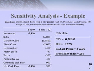
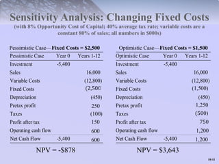
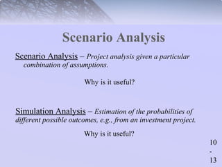
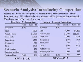
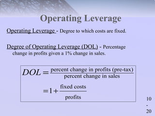
McGraw-Hill/Irwin Copyright © 2012 by The McGraw-Hill Companies, Inc. All rights reserved.
10 
-2 
Project Analysis 
Chapters 8 and 9 develop a framework for project 
analysis. 
This chapter analyzes the robustness of a project’s 
value by asking some “What If” Questions.
10 
-3 
Capital Budget 
Capital Budget – A list of planned investment 
projects.
10 
-4 
Capital Budgeting: 
The Decision Process 
1. Stage 1: The Capital Budget 
2. Stage 2: Project Authorization 
• Outlays required by law or company policy 
• Maintenance or cost reduction 
• Capacity expansion in existing business 
• Investment for new products
10 
-5 
Potential Capital Budgeting 
Problems 
 Ensuring forecasts are consistent 
 Eliminating conflicts of interest 
 Reducing forecast bias 
 Proper selection criteria (NPV and others)
10 
-6 
What-if Testing 
 Sensitivity Analysis - Analysis of the effects on 
project profitability of changes in sales, costs, etc. 
 Scenario Analysis – Analysis given a particular 
combination of assumptions. 
 Simulation Analysis - Estimation of the 
probabilities of different possible outcomes. 
 Break-Even Analysis - Analysis of the level of 
sales at which the company breaks even.
10 
-7 
Sensitivity Analysis 
Analysis of the effects on project profitability of 
changes in sales, costs, etc. 
Why is sensitivity analysis useful?
Base Case: Expected cash flows from a new project (with 8% Opportunity Cost of Capital; 40% 
10 
-8 
Sensitivity Analysis - Example 
average tax rate; variable costs are a constant 80% of sales; all numbers in $000s) 
Year 0 Years 1-12 
Investment -5,400 
Sales 16,000 
Variable Costs (12,800) 
Fixed Costs (2,000) 
Depreciation (450) 
Pretax profit 750 
Taxes (300) 
Profit after tax 450 
Operating cash flow 900 
Net Cash Flow -5,400 900 
Calculate: 
NPV = 
$1,382.47 
IRR = 
12.7% 
Payback Period = 
6 years 
Profitability Index = 
.256
10 
-9 
Sensitivity Analysis - Example 
Possible Range of Variables 
Range 
Pessimistic Expected Optimistic 
Variable 
Sales 14,000 16,000 18,000 
Fixed Costs 2,500 2,000 1,500
Optimistic Case Year 0 Years 1-12 
Investment -5,400 
Sales 18,000 
Variable Costs 
Fixed Costs (2,000) 
Depreciation (450) 
Pretax profit 
Taxes 
Profit after tax 
Operating cash flow 
Net Cash Flow -5,400 
1100--1100 
Sensitivity Analysis: Changing Sales 
(with 8% Opportunity Cost of Capital; 40% average tax rate; variable costs are a 
constant 80% of sales; all numbers in $000s) 
Pessimistic Case—Sales = $14,000 Optimistic Case—Sales = $18,000 
Pessimistic Case Year 0 Years 1-12 
Investment -5,400 
Sales 14,000 
Variable Costs 
Fixed Costs (2,000) 
Depreciation (450) 
Pretax profit 
Taxes 
Profit after tax 
Operating cash flow 
Net Cash Flow -5,400 
NPV = -$426 NPV = $3,191
Sensitivity Analysis: Changing Fixed Costs 
(with 8% Opportunity Cost of Capital; 40% average tax rate; variable costs are a 
Optimistic Case Year 0 Years 1-12 
Investment -5,400 
Sales 16,000 
Variable Costs (12,800) 
Fixed Costs 
Depreciation (450) 
Pretax profit 
Taxes 
Profit after tax 
Operating cash flow 
Net Cash Flow -5,400 
1100--1111 
constant 80% of sales; all numbers in $000s) 
Pessimistic Case—Fixed Costs = $2,500 Optimistic Case—Fixed Costs = $1,500 
Pessimistic Case Year 0 Years 1-12 
Investment -5,400 
Sales 16,000 
Variable Costs (12,800) 
Fixed Costs 
Depreciation (450) 
Pretax profit 
Taxes 
Profit after tax 
Operating cash flow 
Net Cash Flow -5,400 
NPV = -$878 NPV = $3,643
10 
- 
12 
Limits to Sensitivity Analysis 
• Ambiguous 
• How do you consistently define “optimistic” or 
“pessimistic”? 
• Interrelatedness of variables
10 
- 
13 
Scenario Analysis 
Scenario Analysis – Project analysis given a particular 
combination of assumptions. 
Why is it useful? 
Simulation Analysis – Estimation of the probabilities of 
different possible outcomes, e.g., from an investment project. 
Why is it useful?
Scenario Analysis: Introducing Competition 
Assume that it will take two years for competition to enter the market. At this 
time, sales drop 10% and variable costs increase to 82% (increased labor demand). 
What happens to NPV under this scenario? 
1100--1144 
Base Case – No Competition Scenario – Introduce Competition 
Year 0 Years 1-2 Years 3-12 
Investment -5,400 
Sales 16,000 
Variable Costs (12,800) 
Fixed Costs (2,000) (2,000) 
Depreciation (450) (450) 
Pretax profit 750 
Taxes (300) 
Profit after tax 450 
Operating cash flow 900 
Net Cash Flow -5,400 900 
Year 0 Years 1-12 
Investment -5,400 
Sales 16,000 
Variable Costs (12,800) 
Fixed Costs (2,000) 
Depreciation (450) 
Pretax profit 750 
Taxes (300) 
Profit after tax 450 
Operating cash flow 900 
Net Cash Flow -5,400 900 
NPV = $1,382 NPV = -$717 
14,400
10 
- 
15 
Break-Even Analysis 
Break-Even Analysis - Analysis of the level of sales 
at which the project breaks even. 
Why is this useful?
10 
- 
16 
Break-Even Analysis – Example 
(with 8% Opportunity Cost of Capital; 40% average tax rate; variable 
costs are a constant 80% of sales; all numbers in $000s) 
Year 0 Years 1-12 
Investment $5,400 
Sales 45 
´ 
X 
Var. Cost (36 ´ 
X 
) 
Fixed Costs (2,000) 
Depreciation (450) 
Pretax Profit 9 ´ X 
- 
2, 450 
Taxes (40%) 3.6 ´ X 
- 
980 
Net Profit 5.4 ´ X 
- 
1, 470 
Net Cash Flow -5,400 5.4 ´ X 
- 
1,020 
Number X = of Units Sold 
-Determine the number of units 
that must be sold in order to break 
even, on an NPV basis. 
-Suppose each unit has a price 
point of $45,000 
-All other variables are at their 
base case levels
1100--1177 
Break-Even Point: Accounting 
Break-Even Point (Accounting) - The break-even point is the number of units 
sold where net profits = $0. 
= ´ X - 
= = 
0 5.4 1, 470 
X 1, 470 273 Units 
5.4 
What does the accounting break-even point not account for? 
Note: Accounting Break-Even can be expressed in terms of revenue: 
Break-Even level of revenues = fixed costs + depreciation 
additional profit from each additional dollar of sales
10 
- 
18 
Break-Even Point: Finance 
NPV Break-Even Point (Finance): 
How can we find the present value of future cash flows? As long as cash 
flows are equal each year, we can use the Annuity Factor. 
Step 1: PV (Cash Flows) = Annuity Factor Yearly Cash Flows 
r t 
r 
where Annuity Factor = 1- (1 ) 
- 
´ 
+ 
- + - ´ ´ - 
1 (1 .08) 12 Example: PV(Cash Flows) = [5.4 1,020] 
.08 
X
1100--1199 
Break-Even Analysis 
Recall: the break-even point is the number of units sold where NPV = $0. 
Step 2: PV (Cash Flows) = Initial Investment 
- + - ´ ´ - = 
1 (1 .08) 12 Example- [5.4 1,020] 5,400 
.08 
322units 
X 
X 
=
10 
- 
20 
Operating Leverage 
Operating Leverage - Degree to which costs are fixed. 
Degree of Operating Leverage (DOL) - Percentage 
change in profits given a 1% change in sales. 
percent change in profits (pre-tax) 
percent change in sales 
fixed costs 
profits 
1 
DOL 
= 
= +
10 
- 
21 
Operating Leverage: 
Why is it useful?
1100--2222 
Degree of Operating Leverage: 
Example 
Base Case Year 0 Years 1-12 
Investment -5,400 
Sales 16,000 
Variable Costs (12,800) 
Fixed Costs (2,000) 
Depreciation (450) 
Pretax profit 750 
Taxes (300) 
Profit after tax 450 
Operating cash flow 900 
Net Cash Flow -5,400 900 
Optimisic Sales Year 0 Years 1-12 
Investment -5,400 
Sales 18,000 
Variable Costs (14,400) 
Fixed Costs (2,000) 
Depreciation (450) 
Pretax profit 1,150 
Taxes (460) 
Profit after tax 690 
Operating cash flow 1,140 
Net Cash Flow -5,400 1,140 
- = - = 
% Change in Profits = New Old 1,150 750 .5333 
Old 750 
- = 
% Change in Sales = 18,000 16,000 .1250 
16,000 
DOL = % Change in Profits = .5333 = 
4.27 
% Change in Sales .1250
10 
- 
23 
Real Options 
1. Option to expand 
2. Option to abandon 
3. Timing option 
4. Flexible production facilities
10 
- 
24 
Real Options & the Value of 
Flexibility 
Decision Trees – Diagram of sequential decisions and 
possible outcomes. 
 Decision trees help companies determine their options by 
showing various choices and outcomes. 
 The option to avoid a loss or produce extra profit has value. 
 The ability to create an option has value that can be bought or 
sold.
10 
- 
25 
Decision Trees: Example 
NPV=0 
Test New Product 
(Invest $200,000) 
Don’t Test New 
Product 
Success 
Failure 
Pursue project 
NPV=$2million 
Stop project 
NPV=0

Chap010

  • 1.
    McGraw-Hill/Irwin Copyright ©2012 by The McGraw-Hill Companies, Inc. All rights reserved.
  • 2.
    10 -2 ProjectAnalysis Chapters 8 and 9 develop a framework for project analysis. This chapter analyzes the robustness of a project’s value by asking some “What If” Questions.
  • 3.
    10 -3 CapitalBudget Capital Budget – A list of planned investment projects.
  • 4.
    10 -4 CapitalBudgeting: The Decision Process 1. Stage 1: The Capital Budget 2. Stage 2: Project Authorization • Outlays required by law or company policy • Maintenance or cost reduction • Capacity expansion in existing business • Investment for new products
  • 5.
    10 -5 PotentialCapital Budgeting Problems  Ensuring forecasts are consistent  Eliminating conflicts of interest  Reducing forecast bias  Proper selection criteria (NPV and others)
  • 6.
    10 -6 What-ifTesting  Sensitivity Analysis - Analysis of the effects on project profitability of changes in sales, costs, etc.  Scenario Analysis – Analysis given a particular combination of assumptions.  Simulation Analysis - Estimation of the probabilities of different possible outcomes.  Break-Even Analysis - Analysis of the level of sales at which the company breaks even.
  • 7.
    10 -7 SensitivityAnalysis Analysis of the effects on project profitability of changes in sales, costs, etc. Why is sensitivity analysis useful?
  • 8.
    Base Case: Expectedcash flows from a new project (with 8% Opportunity Cost of Capital; 40% 10 -8 Sensitivity Analysis - Example average tax rate; variable costs are a constant 80% of sales; all numbers in $000s) Year 0 Years 1-12 Investment -5,400 Sales 16,000 Variable Costs (12,800) Fixed Costs (2,000) Depreciation (450) Pretax profit 750 Taxes (300) Profit after tax 450 Operating cash flow 900 Net Cash Flow -5,400 900 Calculate: NPV = $1,382.47 IRR = 12.7% Payback Period = 6 years Profitability Index = .256
  • 9.
    10 -9 SensitivityAnalysis - Example Possible Range of Variables Range Pessimistic Expected Optimistic Variable Sales 14,000 16,000 18,000 Fixed Costs 2,500 2,000 1,500
  • 10.
    Optimistic Case Year0 Years 1-12 Investment -5,400 Sales 18,000 Variable Costs Fixed Costs (2,000) Depreciation (450) Pretax profit Taxes Profit after tax Operating cash flow Net Cash Flow -5,400 1100--1100 Sensitivity Analysis: Changing Sales (with 8% Opportunity Cost of Capital; 40% average tax rate; variable costs are a constant 80% of sales; all numbers in $000s) Pessimistic Case—Sales = $14,000 Optimistic Case—Sales = $18,000 Pessimistic Case Year 0 Years 1-12 Investment -5,400 Sales 14,000 Variable Costs Fixed Costs (2,000) Depreciation (450) Pretax profit Taxes Profit after tax Operating cash flow Net Cash Flow -5,400 NPV = -$426 NPV = $3,191
  • 11.
    Sensitivity Analysis: ChangingFixed Costs (with 8% Opportunity Cost of Capital; 40% average tax rate; variable costs are a Optimistic Case Year 0 Years 1-12 Investment -5,400 Sales 16,000 Variable Costs (12,800) Fixed Costs Depreciation (450) Pretax profit Taxes Profit after tax Operating cash flow Net Cash Flow -5,400 1100--1111 constant 80% of sales; all numbers in $000s) Pessimistic Case—Fixed Costs = $2,500 Optimistic Case—Fixed Costs = $1,500 Pessimistic Case Year 0 Years 1-12 Investment -5,400 Sales 16,000 Variable Costs (12,800) Fixed Costs Depreciation (450) Pretax profit Taxes Profit after tax Operating cash flow Net Cash Flow -5,400 NPV = -$878 NPV = $3,643
  • 12.
    10 - 12 Limits to Sensitivity Analysis • Ambiguous • How do you consistently define “optimistic” or “pessimistic”? • Interrelatedness of variables
  • 13.
    10 - 13 Scenario Analysis Scenario Analysis – Project analysis given a particular combination of assumptions. Why is it useful? Simulation Analysis – Estimation of the probabilities of different possible outcomes, e.g., from an investment project. Why is it useful?
  • 14.
    Scenario Analysis: IntroducingCompetition Assume that it will take two years for competition to enter the market. At this time, sales drop 10% and variable costs increase to 82% (increased labor demand). What happens to NPV under this scenario? 1100--1144 Base Case – No Competition Scenario – Introduce Competition Year 0 Years 1-2 Years 3-12 Investment -5,400 Sales 16,000 Variable Costs (12,800) Fixed Costs (2,000) (2,000) Depreciation (450) (450) Pretax profit 750 Taxes (300) Profit after tax 450 Operating cash flow 900 Net Cash Flow -5,400 900 Year 0 Years 1-12 Investment -5,400 Sales 16,000 Variable Costs (12,800) Fixed Costs (2,000) Depreciation (450) Pretax profit 750 Taxes (300) Profit after tax 450 Operating cash flow 900 Net Cash Flow -5,400 900 NPV = $1,382 NPV = -$717 14,400
  • 15.
    10 - 15 Break-Even Analysis Break-Even Analysis - Analysis of the level of sales at which the project breaks even. Why is this useful?
  • 16.
    10 - 16 Break-Even Analysis – Example (with 8% Opportunity Cost of Capital; 40% average tax rate; variable costs are a constant 80% of sales; all numbers in $000s) Year 0 Years 1-12 Investment $5,400 Sales 45 ´ X Var. Cost (36 ´ X ) Fixed Costs (2,000) Depreciation (450) Pretax Profit 9 ´ X - 2, 450 Taxes (40%) 3.6 ´ X - 980 Net Profit 5.4 ´ X - 1, 470 Net Cash Flow -5,400 5.4 ´ X - 1,020 Number X = of Units Sold -Determine the number of units that must be sold in order to break even, on an NPV basis. -Suppose each unit has a price point of $45,000 -All other variables are at their base case levels
  • 17.
    1100--1177 Break-Even Point:Accounting Break-Even Point (Accounting) - The break-even point is the number of units sold where net profits = $0. = ´ X - = = 0 5.4 1, 470 X 1, 470 273 Units 5.4 What does the accounting break-even point not account for? Note: Accounting Break-Even can be expressed in terms of revenue: Break-Even level of revenues = fixed costs + depreciation additional profit from each additional dollar of sales
  • 18.
    10 - 18 Break-Even Point: Finance NPV Break-Even Point (Finance): How can we find the present value of future cash flows? As long as cash flows are equal each year, we can use the Annuity Factor. Step 1: PV (Cash Flows) = Annuity Factor Yearly Cash Flows r t r where Annuity Factor = 1- (1 ) - ´ + - + - ´ ´ - 1 (1 .08) 12 Example: PV(Cash Flows) = [5.4 1,020] .08 X
  • 19.
    1100--1199 Break-Even Analysis Recall: the break-even point is the number of units sold where NPV = $0. Step 2: PV (Cash Flows) = Initial Investment - + - ´ ´ - = 1 (1 .08) 12 Example- [5.4 1,020] 5,400 .08 322units X X =
  • 20.
    10 - 20 Operating Leverage Operating Leverage - Degree to which costs are fixed. Degree of Operating Leverage (DOL) - Percentage change in profits given a 1% change in sales. percent change in profits (pre-tax) percent change in sales fixed costs profits 1 DOL = = +
  • 21.
    10 - 21 Operating Leverage: Why is it useful?
  • 22.
    1100--2222 Degree ofOperating Leverage: Example Base Case Year 0 Years 1-12 Investment -5,400 Sales 16,000 Variable Costs (12,800) Fixed Costs (2,000) Depreciation (450) Pretax profit 750 Taxes (300) Profit after tax 450 Operating cash flow 900 Net Cash Flow -5,400 900 Optimisic Sales Year 0 Years 1-12 Investment -5,400 Sales 18,000 Variable Costs (14,400) Fixed Costs (2,000) Depreciation (450) Pretax profit 1,150 Taxes (460) Profit after tax 690 Operating cash flow 1,140 Net Cash Flow -5,400 1,140 - = - = % Change in Profits = New Old 1,150 750 .5333 Old 750 - = % Change in Sales = 18,000 16,000 .1250 16,000 DOL = % Change in Profits = .5333 = 4.27 % Change in Sales .1250
  • 23.
    10 - 23 Real Options 1. Option to expand 2. Option to abandon 3. Timing option 4. Flexible production facilities
  • 24.
    10 - 24 Real Options & the Value of Flexibility Decision Trees – Diagram of sequential decisions and possible outcomes.  Decision trees help companies determine their options by showing various choices and outcomes.  The option to avoid a loss or produce extra profit has value.  The ability to create an option has value that can be bought or sold.
  • 25.
    10 - 25 Decision Trees: Example NPV=0 Test New Product (Invest $200,000) Don’t Test New Product Success Failure Pursue project NPV=$2million Stop project NPV=0

Editor's Notes

  • #2 Chapter 10 Learning Objectives 1. Appreciate the practical problems of capital budgeting in large corporations. 2. Use sensitivity, scenario, and break-even analyses to see how project profitability would be affected by an error in your forecasts. 3. Understand why an overestimate of sales is more serious for projects with high operating leverage. 4. Recognize the importance of managerial flexibility in capital budgeting.
  • #3 Chapter 10 Outline How Firms Organize the Investment Process Some “What If” Questions Sensitivity Analysis Scenario Analysis Break Even Analysis Real Options and the Value of Flexibility
  • #4 Capital Budget - The list of planned investment projects.
  • #5 Capital Budget - The list of planned investment projects.
  • #7 Sensitivity Analysis - Analysis of the effects on project profitability of changes in sales, costs, etc. Scenario Analysis - Project analysis given a particular combination of assumptions. Simulation Analysis - Estimation of the probabilities of different possible outcomes. Break-Even Analysis - Analysis of the level of sales at which the company breaks even.
  • #8 Sensitivity Analysis - Analysis of the effects on project profitability of changes in sales, costs, etc.
  • #11 Note: It is recommended for practice that students calculate the other valuation techniques learned in Chapter 8 (IRR, etc)
  • #12 Note: It is recommended for practice that students calculate the other valuation techniques learned in Chapter 8 (IRR, etc)
  • #14 Scenario Analysis - Project analysis given a particular combination of assumptions. Simulation Analysis –Estimation of the probabilities of different possible outcomes, e.g., from an investment project.
  • #16 Break-even Analysis – Analysis of the level of sales at which the project breaks even.
  • #19 NPV break-even point – Level of sales at which project net present value becomes positive.
  • #20 Note: Think back to discussion of economic value added (EVA) in Chapter 4. A project that breaks even on a present value basis will have a positive accounting profit but zero economic value added. In other words, it will just cover all its costs, including the cost of capital. Note: The NPV break-even level of sales will be greater than the accounting break-even level of sales. Why?
  • #21 Operating Leverage – Degree to which costs are fixed. Degree of Operating Leverage (DOL) – Percentage change in profits given a 1% change in sales.
  • #22 Operating Leverage – Degree to which costs are fixed. Degree of Operating Leverage (DOL) – Percentage change in profits given a 1% change in sales.
  • #23 Operating Leverage – Degree to which costs are fixed. Degree of Operating Leverage (DOL) – Percentage change in profits given a 1% change in sales.
  • #24 Real Options – Options to invest in, modify or dispose of a capital investment project
  • #25 Decision Trees – Diagram of sequential decisions and possible outcomes.
  • #26 Decision Trees – Diagram of sequential decisions and possible outcomes.