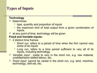
This document provides an overview of production theory concepts. It begins by outlining the chapter objectives, which are to examine a firm's technology, inputs, production process, short and long run production functions, and concepts like isoquants, isocost lines, and technical progress. It then defines production, inputs, and factors of production. Key concepts discussed include production functions, the law of variable proportions, production with one and two variable inputs, isoquants, marginal rate of technical substitution, isocost lines, and producer equilibrium.

1. Chapter 6
Production Theory

2. Chapter Objectives
 To examine the economic analysis of a firm’s technology,




different types of inputs and the process of production.
To help develop an understanding of the distinction between
short run and long run production functions.
To build up a critical appraisal of the law of variable proportions
and returns to scale.
To introduce the concepts of isoquant, isocost line, marginal
rate of technical substitution, elasticity of substitution and
expansion path.
To develop an understanding of technical progress and its
nuances.

3. Production
 Production of goods
All tangible items such as furniture, house, machine, food, car,
etc
 Production of services
 All intangible items like banking, education, management,
consultancy, transportation
 Process of transformation of resources (like land, labour, capital and
entrepreneurship) into goods and services of utility to consumers
&/or producers
 Process of creation of value or wealth through the production of
goods and services that have economic value to either consumers
or other producers
 by change in form (input to output, say steel into car), or
 by change in place (supply chain, say from factory to
dealers/retailer), or
 by changing hands (exchange, say from retailer to consumer)


4. Types of Inputs
Technology
 Determines
 type, quantity and proportion of inputs
 the maximum limit of total output from a given combination of
inputs.
 at any point of time, technology will be given
Fixed and Variable Inputs:
 2 distinct time frames:
 Short run: refers to a period of time when the firm cannot vary
some of its inputs
 Long run: refers to a time period sufficient to vary all of its
inputs, including technology
 Variable input : made to vary in the short run, e.g. raw material,
unskilled/semi skilled labour, etc.
 Fixed input: cannot be varied in the short run, e.g. land, machine,
technology, skill set, etc.

5. Factors of Production
5 factors of production
Land: anything which is gift of nature and not the result of human
effort
Labour: physical or mental effort of human being that undertakes the
production process.
Capital: wealth which is used for further production
Not a gift of nature, but is produced by human beings.
Output of one production process that generally goes as input in
another
Enterprise: ability and action to collect, coordinate, and utilize all the
factors of production for the purpose of economic gains
Also defined as the ability to take risk
Organization: acknowledges a special kind of function
Combination of highly skilled labour and specialized human capital
Organizational efficiency that differentiates one company from
another in terms of success

6. Production Function
 Technological relationship between physical inputs and physical




outputs over a given period of time
Shows the maximum quantity of the commodity that can be
produced per unit of time for each set of alternative inputs, and with
a given level of production technology
Always related to:
 a given time period
 a certain level of technology
Depends upon relation between inputs
Normally a production function is written as:
Q = f (L,K,I,R,E)
(Q is the maximum quantity of output of a good being produced, and
L=labour; K=capital; l=land; R=raw material; E= efficiency
parameter)

7. Production Function with One Variable Input
 Also termed as variable proportion production function
 Short term production function in which production is planned
with one variable input (say L)
 Shows the maximum output a firm can produce when only one of
its inputs can be varied, other inputs remaining fixed
Q = f ( L, K )
where Q = output, L = labour and K = fixed amount of capital
 Total product is a function of labour
TPL = f ( K ,L)
 Average Product (AP) is total product per unit of variable input :
TP
AP =
L
L
 Marginal Product (MP) is addition in total output per unit change
in variable input
MPL =
∆TP
∆L

8. Law of Variable Proportions
Total
Product
(’000
tonnes)
MP
AP
1
20
-
2
50
30
25
3
90
40
30
4
120
30
30
5
140
20
28
6
150
10
25
7
150
0
21.5
8
130
-20
16.25
9
100
-30
Stages
11.1
200
20
Increasing
returns
150
Total Product
(’000 tonnes)
100
Diminishing
returns
Output
Labour
(’00
units)
Marginal
Product
50
Average
Product
0
1 2 3 4 5 6 7 8 9
-50
Labour
Negative
returns
As the quantity of the variable factor is increased with other fixed factors,
the MP and AP of the variable factor will eventually decline.

9. Law of Variable Proportions
Total
Output
C
TPL
B
Panel a
A
Total
Output
O
Labour
Stage I
A*
Panel b
O
Stage II
Stage III
B*
C*
MPL
APL
Labour
Increasing Returns to Variable
Factor
Very first stage
MP>0 and MP>AP
Diminishing Returns to Variable
Factor
2nd stage
MP>0 and MP<AP
Negative Returns
Technically
inefficient
stage
of
production
A rational firm will never operate in this
stage
MP<0 while AP is falling but positive

10. Production Function with 2 Variable Inputs
 In the long run, all the inputs are variable
 Firm has the opportunity to select that combination of inputs
which maximizes returns
 Isoquant
 Locus of all technically efficient combinations (or all possible
factors of production) for producing a given level of output
 Also referred to as iso-product curves
 Taking the production function and fixing level of output Q at
some given quantity, we have an implicit relationship
between units of labour (L) and capital (K)
Q = f ( L, K )

11. Isoquants
Labour (’00
units)
40
6
28
7
18
8
12
9
8
10
Capital (Rs. Crore)
Capital (Rs.
crore)
45
40
35
30
25
20
15
10
5
0
6
7
8
9
10
Labour ('00 units)
An isoquant is the locus of all technically efficient combinations for
producing a given level of output.
Characteristics:
i. Downward sloping
ii. A higher isoquant represents a higher output
iii. Isoquants do not intersect
iv. Convex to the origin

12. Marginal Rate of Technical Substitution
 MRTS measures the reduction in one input due to unit increase
in the other input that is just sufficient to maintain the same level
of output.
∆
K
MRTS LK =
−
∆
L
 MRTS of labour for capital is equal to the slope of the isoquant
 Also equal to the ratio of the marginal product of one input to the
marginal product of other input
∆Q = MPL × ∆L + MPK × ∆K
0 = MPL × ∆ L + MPK × ∆ K
MRTS LK
MPL = − ∆ K
=
MPK
∆L

13. Special Shapes of Isoquants
Capital
Capital
Q3
Q2
Q1
O
Q1
Q2
Q3
Labour
Linear isoquants
Q = f ( L, K ) = aK + bL
Isoquants
are
downward
sloping straight lines, indicating
a constant MRTS
O
Labour
Right angled isoquants
Q =min(
L
,
K
)
α β
Leontief production technology, capital
is a perfect complement for labour, non
existence
of
any
substitutability
between the two factors

14. Isocost Lines
Capital
A2
Panel
a
With wage (w) and interest (r), the total cost
incurred by the firm:
Labour cost (wL) + Capital cost (rK)
A
A1
O
B1 B
B2
Labou
r
C = wL + rK
The isocost line represents the locus of points of all the different combinations of
two inputs that a firm can procure, given the total cost and prices of the inputs.
The (absolute) slope of this line is equal to the ratio of the input prices.
C
∆K
w
Slope = −
= r =
∆L C
r
w

15. Producer’s Equilibrium
Capital
Capital
Panel a
A2
A
A
C
E
K
D
Q0
L*
R
A1
E
K*
O
Panel b
B
Q2
Q1
Q3
S
O
Labour
Maximization of output subject to a
cost constraint
L
B1
B
Q
B2
Labour
Minimization cost for a given level of
output
Necessary condition for equilibrium:
Slope of isoquant = Slope of isocost line