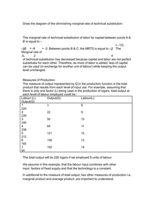
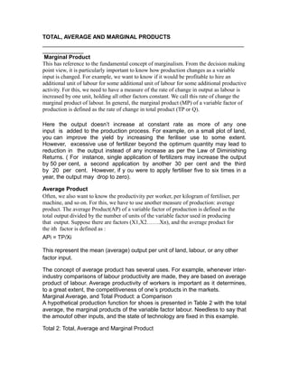
1. UNIT – 3
Production and cost concepts
LESSON 14 PRODUCTION CONCEPT AND ANALYSIS
Learning outcomes
After studying this unit, you should be able to:
Develop a theoretical base for analyzing empirical situation define
the concept and techniques relevant for production decision
analysis
distinguish between demand analysis and production analysis
decision rules for optimum input choice and product mix
INTRODUCTION
This is the first lesson of unit 3. this lesson will give you the whole idea about the
production function and its related concepts.
Production is concerned with the supply side of the market. The basis function of
a firm is that of readying and presenting a product for sale-presumably at a profit.
Production analysis related physical output to physical units of factors
of production. In the production process, various inputs are transformed into
some form of output. Inputs are broadly classified as land, labour,
capital and entrepreneurship (which embodies the managerial functions
of risk taking, organizing, planning, controlling and directing resources). In
production analysis, we study the least-cost combination of factor inputs,
factor productivities and returns to scale.
In this lesson we shall introduce several new concepts to understand the
relationship involved in the production process. We are concerned with economic
efficiency of production which refers to minimization of cost for a given output
level. The efficiency of production process is determined by the proportions in
which various inputs are used, the absolute level of each input and productivity of
each input at various levels. Since inputs have a cost attached, the degree
of efficiency in production gets translated into a level of costs per units of output.
WHY TO STUDY PRODUCTION?
When making the decision of what to produce and what not to produce, the study of
production is needed. The discussion in this lesson covers decision rules for
determining the quantity of various inputs to produce a firm’s output under
different circumstances. It also develops a basis upon which firm’s costs can be
constructed. After all, a firm incurs costs because it must pay for productive
2. factors. Thus an understanding of production helps provide a foundation for the
study of cost.
Business firms produce goods or service as a means to an end. Beside meeting
of final consumer needs, the end objective of a firm may be to maximize profits,
to gain or maintain market share, to achieve a target return on investment, or any
combination there of. In case of public goods, the objective may be to provide a
particular service, such as education and health, within the bounds of a budget
constraint. In other words, a firm attempts to combine various inputs in
such a way that minimum resources are committed to produce a given
product or that maximum production results from a given input. To achieve this,
persons in the decision-making position should have a basis understanding
of the process of production, and also the time perspective of production.
PRODUCTION FUNCTION
A production function expresses the technological or engineering
relationship between the output of product and its inputs. In other words,
the relationship between the amount of various inputs used in the
production process and the level of output is called a production function
Traditional economic theory talks about land, labour, capital and organization or
management as the four major factors of production. Technology also contributes
to output growth as the productivity of the factors of production depends on the
state of technology. The point which needs to be emphasized here is that
the production function describes only efficient levels of output; that is the
output associated with each combination of inputs is the maximum output
possible, given the existing level of technology. Production function
changes as the technology changes.
Production function is represented as follows:
Q=f(f1, f2,……fn);
Where f1, f2,…..fn are amounts of various inputs such as land, labour, capital etc., and Q
is the level of output for a firm. This is a positive functional relationship implying that the
output varies in the same direction as the input quantity. In other words, if all the other
inputs are held constant, output will go up if the quantity of one input is increased. This
means that the partial derivative of Q with respect to each of the inputs is greater than
zero. However, for a reasonably good understanding of production decision problems, it
is convenient to work with two factors of production. If labour (L) and capital(K) are the
only two factors, the production function reduces to:
Q=f(K,L)
From the above relationship, it is easy to infer that for a given value of Q,
alternative combinations of K and L can be used. It is possible because labour
3. and capital are substitutes to each other to some extent. However, a
minimum amount of labour and capital is absolutely essential for the
production of a commodity. Thus for any given level of Q, an entrepreneur will
need to hire both labour and capital but he will have the option to use the two
factors in any one of the many possible combinations.
For example, in an automobile assembly plant, it is possible to substitute,
to some extent, the machine hours by man hours to achieve a particular
level of output (no. of vehicles). The alternative combinations of factors for a
given output level will be such that if the use of one factor input is
increased, the use of another factor will decrease, and vice versa.
ISOQUANTS
Isoquants are a geometric representation of the production function. It is also
known as the ISO PRODUCT curve. As discussed earlier, the same level of
output can be produced by various combinations of factor inputs. Assuming
continuous variation in the possible combination of labor and capital, we can
draw a curve by plotting all these alternative combinations for a given level
of output. This curve which is the locus of all possible combinations is called
Isoquants or Iso-product curve. Each Isoquants corresponds to a specific level of
output and shows different ways all technologically efficient, of producing
that quantity of outputs. The Isoquants are downward slopping and convex
to the origin. The curvature (slope) of an Isoquants is significant because
it indicates the rate at which factors K&L can be substituted for each other while
a constant level of output of maintained. As we proceed north-eastward from the
origin, the output level corresponding to each successive isoquant
increases, as a higher level of output usually requires greater amounts of the
two inputs. Two Isoquants don’t intersect each other as it is not possible to
have two output levels for a particular input combination.
Draw an isoquant curve on the basis of above considerations:
Marginal Rate if Technical Substitution:
It can be called as MRTS. MRTS is defined
as the rate at which two factors are substituted for each other. Assuming that 10
pairs of shoes can be produced in the following three ways.
Q K L
10 8 2
10 4 4
10 2 8
two factors by plotting these
We can derive the MRTS between the combinations along a curve (Isoquant).
4. Draw the diagram of the diminishing marginal rate of technical substitution:
The marginal rate of technical substitution of labor for capital between points A &
B is equal to –
= -1/2.
-∆K = -4 = -2. Between points B & C, the MRTS is equal to –2 The
Marginal rate of
∆L 2 4
of technical substitution has decreased because capital and labor are not perfect
substitutes for each other. Therefore, as more of labor is added, less of capital
can be used (in exchange for another unit of labour) while keeping the output
level unchanged.
Measures of Production
The measure of output represented by Q in the production function is the total
product that results from each level of input use. For example, assuming that
there is only one factor (L) being used in the production of cigars, total output at
each level of labour employed could be :
Labour (L) Output(Q) Labour(L)
Output(Q)
1 3 8
220
2 22 9
239
3 50 10
246
4 84 11
238
5 121 12
212
6 158 13
165
7 192 14
94
The total output will be 220 cigars if we employed 8 units of labour.
We assume in this example, that the labour input combines with other
input factors of fixed supply and that the technology is a constant.
In additional to the measure of total output, two other measures of production i.e.
marginal product and average product, are important to understand.
5. TOTAL, AVERAGE AND MARGINAL PRODUCTS
________________________________________________________________
_____________
Marginal Product
This has reference to the fundamental concept of marginalism. From the decision making
point view, it is particularly important to know how production changes as a variable
input is changed. For example, we want to know if it would be profitable to hire an
additional unit of labour for some additional unit of labour for some additional productive
activity. For this, we need to have a measure of the rate of change in output as labour is
increased by one unit, holding all other factors constant. We call this rate of change the
marginal product of labour. In general, the marginal product (MP) of a variable factor of
production is defined as the rate of change in total product (TP or Q).
Here the output doesn’t increase at constant rate as more of any one
input is added to the production process. For example, on a small plot of land,
you can improve the yield by increasing the feriliser use to some extent.
However, excessive use of fertilizer beyond the optimum quantity may lead to
reduction in the output instead of any increase as per the Law of Diminishing
Returns. ( For instance, single application of fertilizers may increase the output
by 50 per cent, a second application by another 30 per cent and the third
by 20 per cent. However, if y ou were to apply fertiliser five to six times in a
year, the output may drop to zero).
Average Product
Often, we also want to know the productivity per worker, per kilogram of fertiliser, per
machine, and so on. For this, we have to use another measure of production: average
product. The average Product(AP) of a variable factor of production is defined as the
total output divided by the number of units of the variable factor used in producing
that output. Suppose there are factors (X1,X2…….Xn), and the average product for
the ith factor is defined as :
APi = TP/Xi
This represent the mean (average) output per unit of land, labour, or any other
factor input.
The concept of average product has several uses. For example, whenever inter-
industry comparisons of labour productivity are made, they are based on average
product of labour. Average productivity of workers is important as it determines,
to a great extent, the competitiveness of one’s products in the markets.
Marginal Average, and Total Product: a Comparison
A hypothetical production function for shoes is presented in Table 2 with the total
average, the marginal products of the variable factor labour. Needless to say that
the amoutof other inputs, and the state of technology are fixed in this example.
Total 2: Total, Average and Marginal Product
6. ________________________________________________________________
_____________
Labour Input Total Output Average Marginal
(L) (TP) Products Product
(AP = TP/L) MP =
∆TP
∆L
0 0 0 0
1 14 14 14
2 52 26 38
3 108 36 56
4 176 44 68
5 250 50 74
6 324 54 74
7 392 56 68
8 448 56 56
9 486 54 38
10 500 50 14
11 484 44 -16
12 432 36 -52
13 338 26 -94
14 196 14 -142
________________________________________________________________
_____________
The value for marginal product are written between each increment of labour
input because those e values represent the marginal productivity over
the respective intervals.
In both the table and the graphic representation, we see that both
average and marginal products first increase, reach the maximum, and
eventually decline. Note that MP=AP at the maximum of the average product
function. This is always the case. If MP>AP, the average will be pushed
up by the incremental unit, and if MP<AP, the average will be pulled
down. It follows that the average product will reach its peak where MP=AP.
Elasticity of Production
This is a concept which is based on the relationship between Average Product
(AP) and Marginal Product (MP). The elasticity of production (eq) is defined as
the rate of fractional change in total product, ∆ Q
∆L
7. ------- - relative to a slight fractional change in a variable factor, say
labour, ------- - .
Thus
Q
L
∆Q/Q ∆Q L ∆ Q/ ∆ L MPL
1
e q =
= . = =
∆L/L ∆L Q Q/L APL
1
Thus labour elasticity of Production, e q is the ratio of marginal productivity of
labour to average productivity of labour. In the same way, you may find that
capital elasticity of production is simply the ratio of marginal productivity to
average productivities of capital. Sometimes, such concepts are renamed as
input elasticity of output. In an estimated production function, the aggregate of
input elasticities is termed as the function coefficient.
Elasticity of Factor Substitution
This is another concepts of elasticity which has a tremendous practical use in the
f
context of production analysis. The elasticity of factor substitution, e s, is
a measure of ease with which
the varying factors can be substituted for others; it is the percentage change in
factor production
K
rate of technical
( ) with respect to a given change in marginal substitution
between factors
L
(MRTS KL).
Thus,
∆(K/L) (MRTS KL)
f
es .
=
(K/L) ∆(MRTS KL)
∆(K/L)
∆(MRTS KL)
= .
(K/L)
∆(MRTSKL)
∆(K/L) (MPK/MPL)
= .
∆(MPK/MP
L)
(K/L)
The elasticity coefficient of factor substitution, s, differs depending upon
1
e the
form of production function. You should be able to see now that factor intensity
(factor ratio), factor productivity, factor elasticity and elasticity of factor
8. substitution are all related concepts in the context of production analysis.
Slide 4
Total product
Total product means a total quantity of
outputou that is producedod by a firm with use
of theth given inputsts.
Slide 5 Averagea
g product
It is definedfine as the total output divided byby
theth number of units of theth variable factor
used inin producinging that output.
Formula of average product:
AP = TP / Xi
Where AP = averageavag product;
TPTP = total product
Xi = n number of factorsfa.
Slide 6
Marginalrgi productpr
Meaning :
it isis thethe totalto
increasecr in a
productivity because of the increase in the
productionon of one more unit.
product
Formula of marginalmargi :
MP = changege in total productprouc /
change in quantity
___________________________________
___________________________________
___________________________________
10. Slide 7 ___________________________________
___________________________________
___________________________________
___________________________________
___________________________________
___________________________________
___________________________________
Stages of production
There are threeth stages of production:
1. In it the average product is rising thoughth
the
marginalma productuct has begungun to fall
2. In it average productuct is maximummamum and it
ends at a point where marginalal product
is zero.
3. In it marginal product is negative
11. Slide 7 ___________________________________
___________________________________
___________________________________
___________________________________
___________________________________
___________________________________
___________________________________
Stages of production
There are threeth stages of production:
1. In it the average product is rising thoughth
the
marginalma productuct has begungun to fall
2. In it average productuct is maximummamum and it
ends at a point where marginalal product
is zero.
3. In it marginal product is negative
12. Slide 7 ___________________________________
___________________________________
___________________________________
___________________________________
___________________________________
___________________________________
___________________________________
Stages of production
There are threeth stages of production:
1. In it the average product is rising thoughth
the
marginalma productuct has begungun to fall
2. In it average productuct is maximummamum and it
ends at a point where marginalal product
is zero.
3. In it marginal product is negative