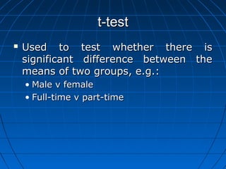
Data Analysis Using
SPSS
t-test
t-test


Used to test whether there is
significant difference between the
means of two groups, e.g.:
• Male v female
• Full-time v part-time
t-test


Typical hypotheses for t-test:
a) There is no difference in affective
commitment (affcomm) between male
and female employees
b) There is no difference in continuance
commitment (concomm) between male
and female employees
c) There is no difference in normative
commitment (norcomm) between male
and female employees
Performing T-test
Analyze →
Compare Means →
Independent-Samples T-test
Performing T-test


Select the variables to test (Test
Variables), in this case:
• affcomm
• concomm
• norcomm



And bring the variables to the “Test
Variables” box
Performing T-test




Select the grouping variable, i.e.
gender; bring it to the “grouping
variable” box
Click “Define Groups”
Performing T-test



Choose “Use specified values”
Key in the codes for the variable
“gender” as used in the “Value
Labels”. In this case:
1 - Male
2 - Female



Click “Continue”, then “OK”
T-Test: SPSS Output

Group Statistics

affcomm
concomm
norcomm

GENDER OF
RESPONDENT
MALE
FEMALE
MALE
FEMALE
MALE
FEMALE

N
357
315
357
315
357
315

Mean
3.49720
3.38016
3.18838
3.15159
3.24090
3.27540

Std. Deviation
.731988
.696273
.756794
.666338
.665938
.647409

Std. Error
Mean
.038741
.039231
.040054
.037544
.035245
.036477
T-test: SPSS Output

Independent Samples Test
Levene's Test for
Equality of Variances

F
affcomm

concomm

norcomm

Equal variances
assumed
Equal variances
not assumed
Equal variances
assumed
Equal variances
not assumed
Equal variances
assumed
Equal variances
not assumed

Sig.

1.048

t

Sig. (2-tailed)

df

Mean
Difference

Std. Error
Difference

95% Confidence
Interval of the
Difference
Lower
Upper

.656

.418

670

.035

.117040

.055308

.008442

.225638

666.213

.034

.117040

.055135

.008780

.225300

.665

670

.506

.036788

.055335

-.071863

.145440

.670

.021

2.116
2.123

5.353

.306

t-test for Equality of Means

669.997

.503

.036788

.054899

-.071006

.144582

-.679

670

.497

-.034500

.050813

-.134272

.065271

-.680

663.726

.497

-.034500

.050723

-.134097

.065096


From the SPSS output, we are
able to see that the means of the
respective variables for the two
groups are:
• Affective commitment (affcomm)


Male 3.49720 Female 3.38016

• Continuance commitment (concomm)


Male 3.18838 Female 3.15159

• Normative commitment (norcomm)


Male 3.24090 Female 3.27540
T-test: Interpretation


For the variable “affcomm”
• Levene’s Test for Equality of Variances
shows that F (1.048) is not significant
(0.306)* therefore the “Equal variances
assumed” row will be used for the ttest.
* This score (sig.) has to be 0.05 or less to be
considered significant.
T-test: Interpretation




Under the “t-test for Equality of
Means” look at “Sig. (2-tailed)”
for “Equal variances assumed”.
The score is 0.035 (which is less
than 0.05), therefore there is a
significant difference between
the means of the two groups.
T-test: Interpretation

Independent Samples Test
Levene's Test for
Equality of Variances

F
affcomm

concomm

norcomm

Equal variances
assumed
Equal variances
not assumed
Equal variances
assumed
Equal variances
not assumed
Equal variances
assumed
Equal variances
not assumed

Sig.

1.048

t

Sig. (2-tailed)

df

Mean
Difference

Std. Error
Difference

95% Confidence
Interval of the
Difference
Lower
Upper

.656

.418

670

.035

.117040

.055308

.008442

.225638

666.213

.034

.117040

.055135

.008780

.225300

.665

670

.506

.036788

.055335

-.071863

.145440

.670

.021

2.116
2.123

5.353

.306

t-test for Equality of Means

669.997

.503

.036788

.054899

-.071006

.144582

-.679

670

.497

-.034500

.050813

-.134272

.065271

-.680

663.726

.497

-.034500

.050723

-.134097

.065096
T-test: Interpretation


For the variable “concomm”
• Levene’s Test for Equality of Variances
shows that F (5.353) is significant
(0.021)* therefore the “Equal variances
not assumed” row will be used for the ttest.
* This score (sig.) is less than 0.05, so there
is significant different in the variances of the
two groups.
T-test: Interpretation




Under the “t-test for Equality of
Means” look at “Sig. (2-tailed)” for
“Equal variances not assumed”.
The score is 0.503 (which is more
than 0.05), therefore there is no
significant difference between the
means of the two groups.
T-test: Interpretation
Independent Samples Test
Levene's Test for
Equality of Variances

F
affcomm

concomm

norcomm

Equal variances
assumed
Equal variances
not assumed
Equal variances
assumed
Equal variances
not assumed
Equal variances
assumed
Equal variances
not assumed

Sig.

1.048

t

Sig. (2-tailed)

df

Mean
Difference

Std. Error
Difference

95% Confidence
Interval of the
Difference
Lower
Upper

.656

.418

670

.035

.117040

.055308

.008442

.225638

666.213

.034

.117040

.055135

.008780

.225300

.665

670

.506

.036788

.055335

-.071863

.145440

.670

.021

2.116
2.123

5.353

.306

t-test for Equality of Means

669.997

.503

.036788

.054899

-.071006

.144582

-.679

670

.497

-.034500

.050813

-.134272

.065271

-.680

663.726

.497

-.034500

.050723

-.134097

.065096
T-test: Interpretation


For the variable “norcomm”
• Levene’s Test for Equality of Variances
shows that F (0.656) is not significant
(0.418)* therefore the “Equal variances
are assumed” row will be used for the ttest.
* This score (sig.) is more than 0.05, so there
is no significant different in the variances of
the two groups.
T-test: Interpretation




Under the “t-test for Equality of
Means” look at “Sig. (2-tailed)” for
“Equal variances assumed”.
The score is 0.497 (which is more
than 0.05), therefore there is no
significant difference between the
means of the two groups.

T test

  • 1.
  • 2.
    t-test  Used to testwhether there is significant difference between the means of two groups, e.g.: • Male v female • Full-time v part-time
  • 3.
    t-test  Typical hypotheses fort-test: a) There is no difference in affective commitment (affcomm) between male and female employees b) There is no difference in continuance commitment (concomm) between male and female employees c) There is no difference in normative commitment (norcomm) between male and female employees
  • 4.
    Performing T-test Analyze → CompareMeans → Independent-Samples T-test
  • 7.
    Performing T-test  Select thevariables to test (Test Variables), in this case: • affcomm • concomm • norcomm  And bring the variables to the “Test Variables” box
  • 10.
    Performing T-test   Select thegrouping variable, i.e. gender; bring it to the “grouping variable” box Click “Define Groups”
  • 12.
    Performing T-test   Choose “Usespecified values” Key in the codes for the variable “gender” as used in the “Value Labels”. In this case: 1 - Male 2 - Female  Click “Continue”, then “OK”
  • 14.
    T-Test: SPSS Output GroupStatistics affcomm concomm norcomm GENDER OF RESPONDENT MALE FEMALE MALE FEMALE MALE FEMALE N 357 315 357 315 357 315 Mean 3.49720 3.38016 3.18838 3.15159 3.24090 3.27540 Std. Deviation .731988 .696273 .756794 .666338 .665938 .647409 Std. Error Mean .038741 .039231 .040054 .037544 .035245 .036477
  • 15.
    T-test: SPSS Output IndependentSamples Test Levene's Test for Equality of Variances F affcomm concomm norcomm Equal variances assumed Equal variances not assumed Equal variances assumed Equal variances not assumed Equal variances assumed Equal variances not assumed Sig. 1.048 t Sig. (2-tailed) df Mean Difference Std. Error Difference 95% Confidence Interval of the Difference Lower Upper .656 .418 670 .035 .117040 .055308 .008442 .225638 666.213 .034 .117040 .055135 .008780 .225300 .665 670 .506 .036788 .055335 -.071863 .145440 .670 .021 2.116 2.123 5.353 .306 t-test for Equality of Means 669.997 .503 .036788 .054899 -.071006 .144582 -.679 670 .497 -.034500 .050813 -.134272 .065271 -.680 663.726 .497 -.034500 .050723 -.134097 .065096
  • 16.
     From the SPSSoutput, we are able to see that the means of the respective variables for the two groups are: • Affective commitment (affcomm)  Male 3.49720 Female 3.38016 • Continuance commitment (concomm)  Male 3.18838 Female 3.15159 • Normative commitment (norcomm)  Male 3.24090 Female 3.27540
  • 17.
    T-test: Interpretation  For thevariable “affcomm” • Levene’s Test for Equality of Variances shows that F (1.048) is not significant (0.306)* therefore the “Equal variances assumed” row will be used for the ttest. * This score (sig.) has to be 0.05 or less to be considered significant.
  • 18.
    T-test: Interpretation   Under the“t-test for Equality of Means” look at “Sig. (2-tailed)” for “Equal variances assumed”. The score is 0.035 (which is less than 0.05), therefore there is a significant difference between the means of the two groups.
  • 19.
    T-test: Interpretation Independent SamplesTest Levene's Test for Equality of Variances F affcomm concomm norcomm Equal variances assumed Equal variances not assumed Equal variances assumed Equal variances not assumed Equal variances assumed Equal variances not assumed Sig. 1.048 t Sig. (2-tailed) df Mean Difference Std. Error Difference 95% Confidence Interval of the Difference Lower Upper .656 .418 670 .035 .117040 .055308 .008442 .225638 666.213 .034 .117040 .055135 .008780 .225300 .665 670 .506 .036788 .055335 -.071863 .145440 .670 .021 2.116 2.123 5.353 .306 t-test for Equality of Means 669.997 .503 .036788 .054899 -.071006 .144582 -.679 670 .497 -.034500 .050813 -.134272 .065271 -.680 663.726 .497 -.034500 .050723 -.134097 .065096
  • 20.
    T-test: Interpretation  For thevariable “concomm” • Levene’s Test for Equality of Variances shows that F (5.353) is significant (0.021)* therefore the “Equal variances not assumed” row will be used for the ttest. * This score (sig.) is less than 0.05, so there is significant different in the variances of the two groups.
  • 21.
    T-test: Interpretation   Under the“t-test for Equality of Means” look at “Sig. (2-tailed)” for “Equal variances not assumed”. The score is 0.503 (which is more than 0.05), therefore there is no significant difference between the means of the two groups.
  • 22.
    T-test: Interpretation Independent SamplesTest Levene's Test for Equality of Variances F affcomm concomm norcomm Equal variances assumed Equal variances not assumed Equal variances assumed Equal variances not assumed Equal variances assumed Equal variances not assumed Sig. 1.048 t Sig. (2-tailed) df Mean Difference Std. Error Difference 95% Confidence Interval of the Difference Lower Upper .656 .418 670 .035 .117040 .055308 .008442 .225638 666.213 .034 .117040 .055135 .008780 .225300 .665 670 .506 .036788 .055335 -.071863 .145440 .670 .021 2.116 2.123 5.353 .306 t-test for Equality of Means 669.997 .503 .036788 .054899 -.071006 .144582 -.679 670 .497 -.034500 .050813 -.134272 .065271 -.680 663.726 .497 -.034500 .050723 -.134097 .065096
  • 23.
    T-test: Interpretation  For thevariable “norcomm” • Levene’s Test for Equality of Variances shows that F (0.656) is not significant (0.418)* therefore the “Equal variances are assumed” row will be used for the ttest. * This score (sig.) is more than 0.05, so there is no significant different in the variances of the two groups.
  • 24.
    T-test: Interpretation   Under the“t-test for Equality of Means” look at “Sig. (2-tailed)” for “Equal variances assumed”. The score is 0.497 (which is more than 0.05), therefore there is no significant difference between the means of the two groups.