The production function shows the relationship between inputs used in production (capital, labor, land, etc.) and the maximum output that can be produced from those inputs. There are two types of production functions: fixed proportions, where inputs must be used in specific quantities, and variable proportions, where inputs can be varied. The law of variable proportions states that as one variable input is increased, at some point marginal product will increase, then decrease, and eventually become negative. 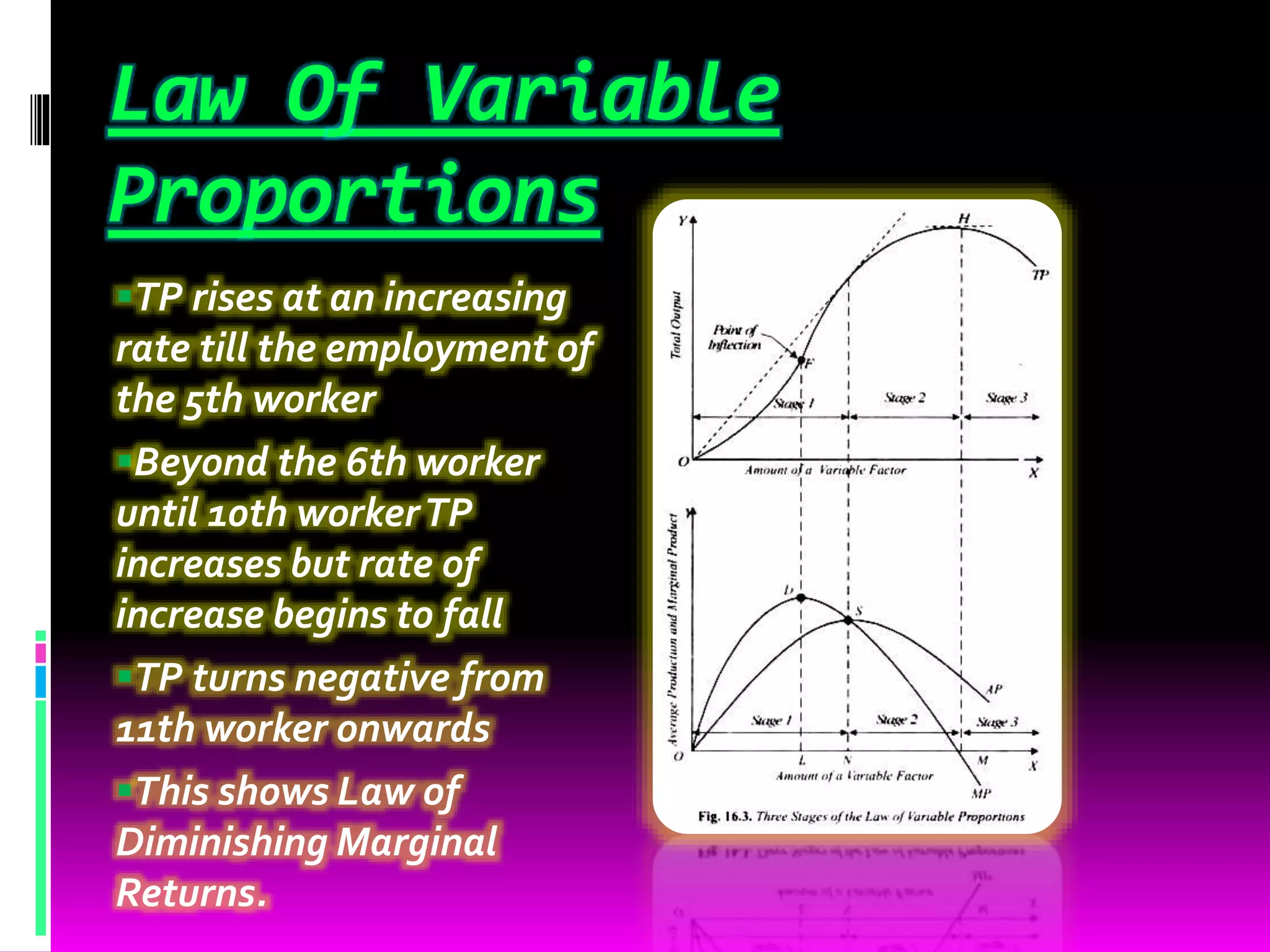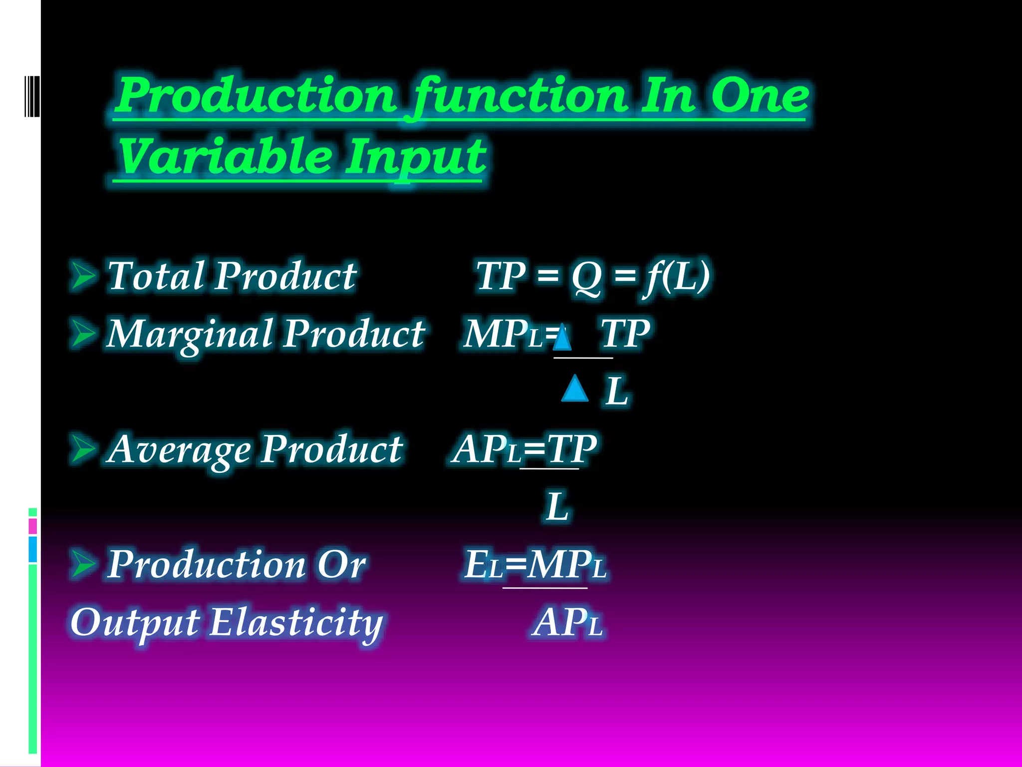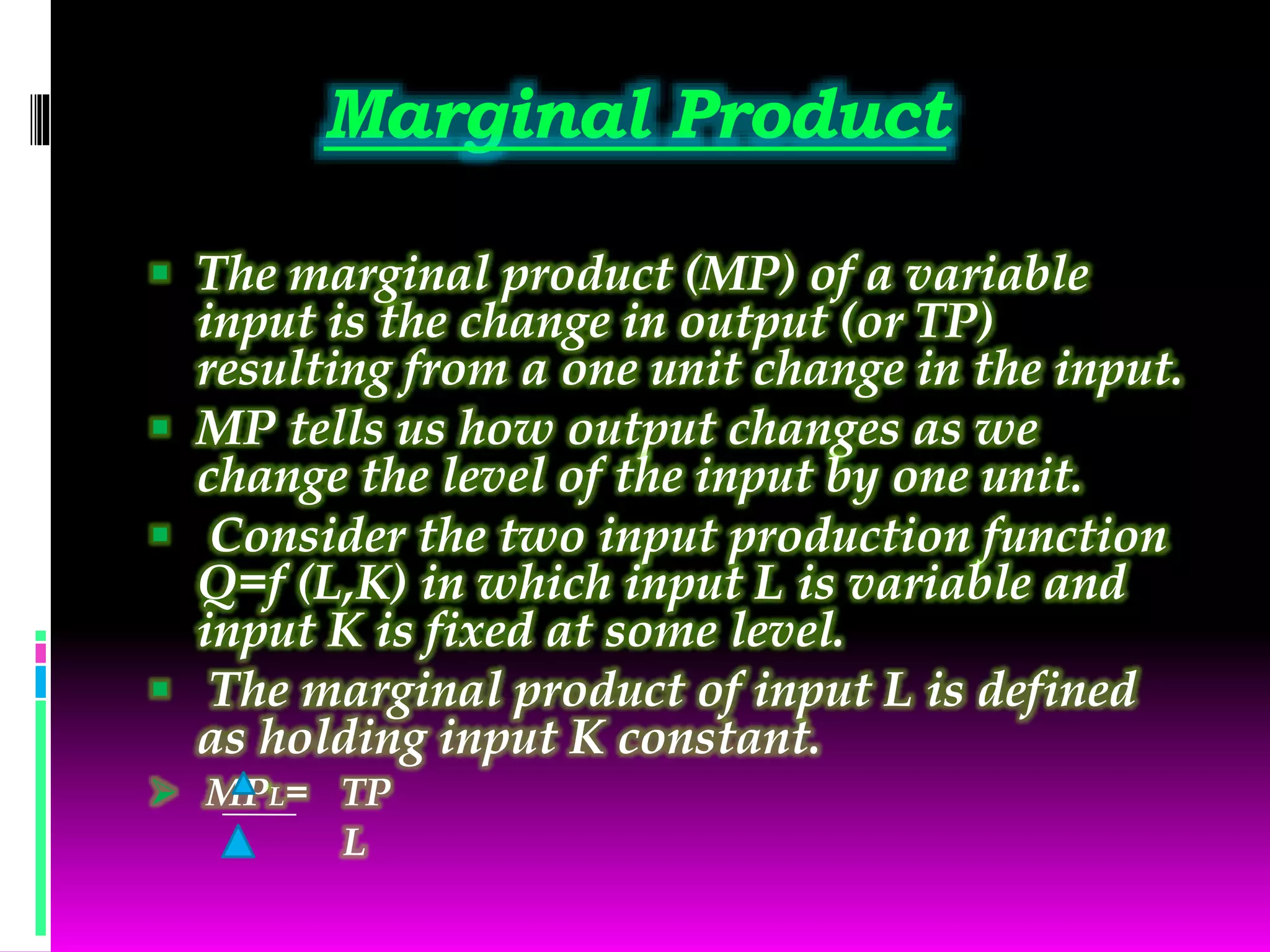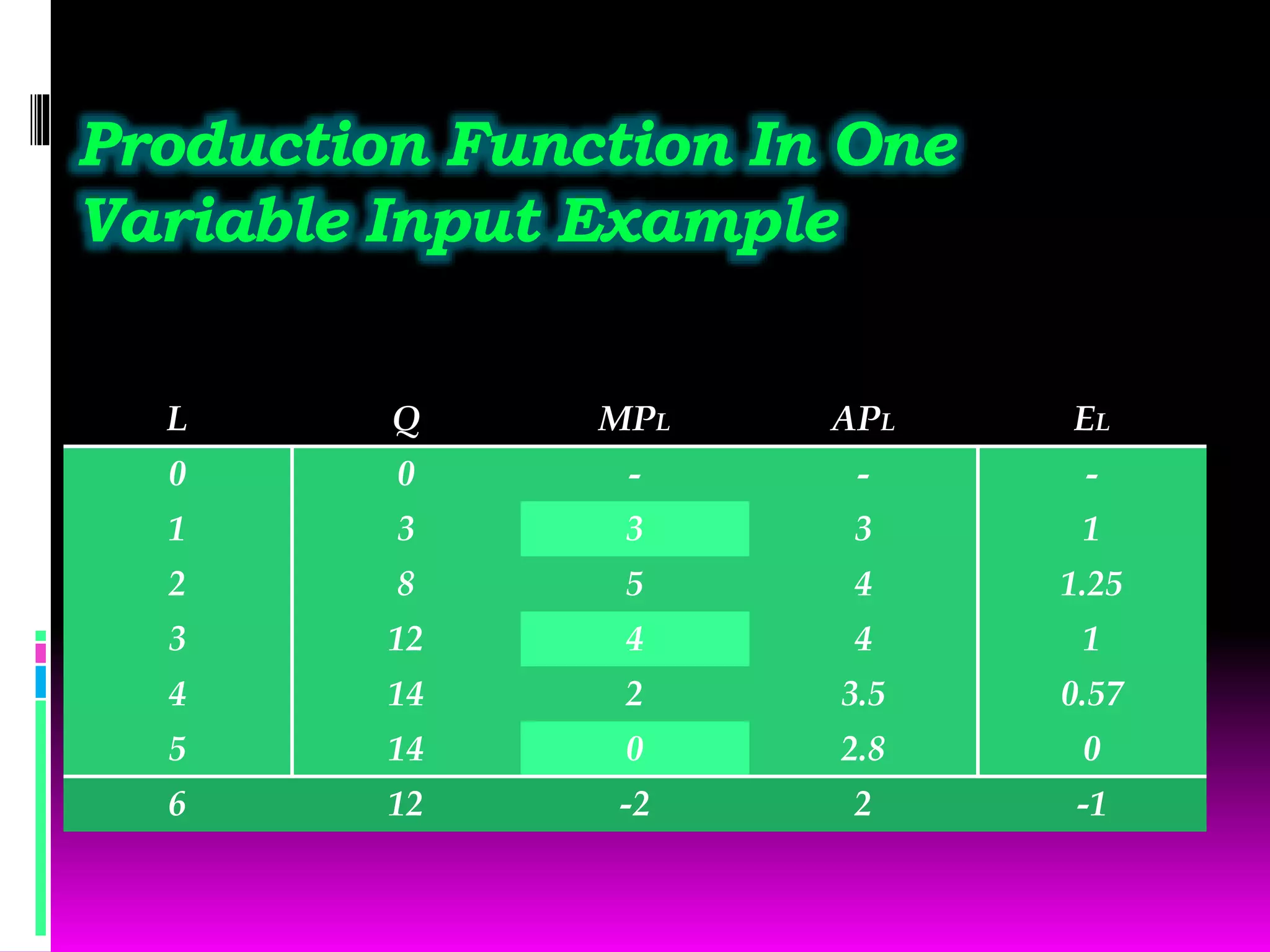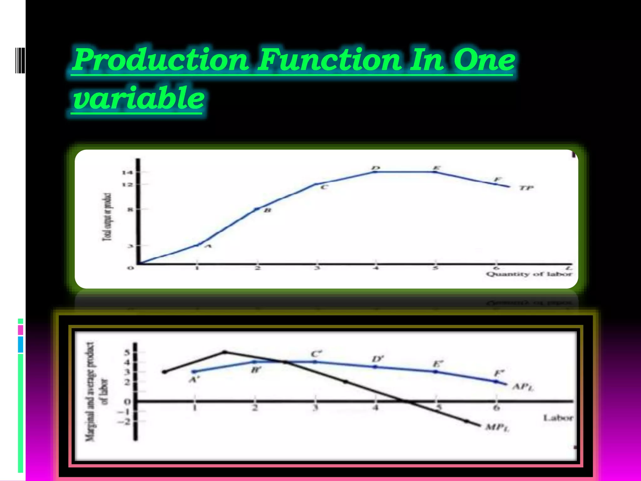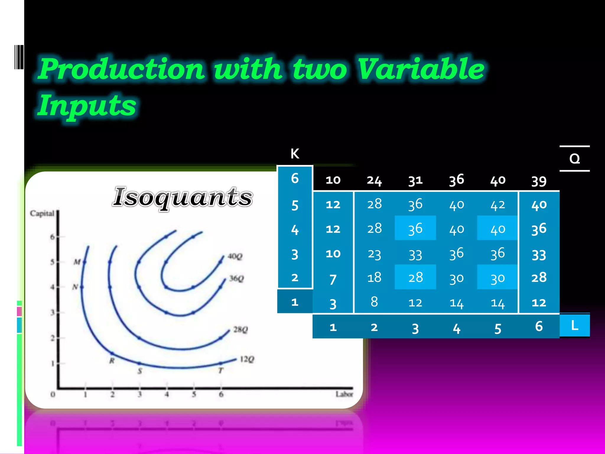A production function with one variable input graphs total product, marginal product, and average product against the input level. A production function with two variable inputs uses isoquants to show combinations of inputs that produce the same output level.

1. PRODUCTION
FUNCTION

2. Table of contents
 Definition and example of Production Function
 Types of Production Function
 Law Of Production Function
 Law of Variable Proportions
 Production Function with one Variable Input
 Production Function with two Variable Inputs

3. Production Function
 Production refers to the transformation of
inputs or resources into outputs of goods and
services. In other words, production refers to all
of the activities involved in the production of
goods and services, from borrowing to set up or
expand production facilities, to hiring workers,
purchasing row materials, running quality
control, cost accounting, and so on, rather than
referring merely to the physical transformation
of inputs into outputs of goods and services.

4. For Example
 A computer company hires workers to use
machinery, parts, and raw materials in
factories to produce personal computers.
 The output of a firm can either be a final
commodity or an intermediate product such
as computer and semiconductor respectively.
 The output can also be a service rather than
a good such as education, medicine, banking
etc.

5. Mathematical Representation
 Mathematical representation of the
relationship:
 Q = f (K, L, La)
  Output (Q) is dependent upon the amount of
capital (K), Land(L) and Labour (La) used

6.  There are two distinct types of production
function that show possible range of
substitution inputs in the production process
 Fixed proportion Production function
 Variable proportions production function

7. Short term
 Time when one input (say, capital)
remains constant and an addition to
output can be obtained only by using
more labour.Long run: Both inputs
become variable.Production process is
subject to various phases-Laws of
production state the relationship between
output and input.

8. Equilibrium Output
 It refers to the level of output where the aggregate
demand is equal to the Aggregate Supply(AD=AS)
in an economy. It signifies that Whatever the
producers intend to produce during the year is
exactly equal to what the buyers intend to buy
during the year.
 Where, AD=C+1(for a two sector economy)
 And AS=C+S
 Where, AD=Aggregate Demand, AS=Aggregate
Supply
 C=Consumption, I=Investment, S=Saving

9. Law of Variable Proportions
 One factor (say, L) is variable and the other
factor (say, K) is constant
 Labour is homogeneous
 Technology remains constant
 Input prices are given

10. Ex ante
 Ex-ante, derived from the Latin for "before the
event," is a term that refers to future events,
such as future returns or prospects of a
company. ... An example of ex-ante analysis is
when an investment company values a stock ex
ante and then compares the predicted results to
the actual movement of the stock's price.

11. Meaning of Ex-ante (Planned)
Aggregate demand:
 In a two sector (Household and Firm) economy,
ex-ante aggregate demand (AD) for final goods
is the sum total of ex-ante consumption
expenditure (C) and ex-ante investment
expenditure (I) on final goods.
 Thus, AD has two determinants (measures) C
and I which are explained below.
 Symbolically:
 AD = C + I

12. Ex-ante Consumption
Expenditure:
 This refers to planned (desired) consumption
expenditure of households. Consumption function is
represented by C = C + by where indicates
autonomous consumption (i.e., consumption
expenditure when income is zero), b shows
marginal propensity to consume (MPC) and Y
stands for level of income. Remember, consumption
demand is the total expenditure which all the
households in the economy are willing to incur on
purchase of goods and services for their personal
satisfaction

13. Ex-ante Investment
Expenditure:
 This refers to planned investment expenditure of private
firms. For simplicity, we assume a constant price and
constant rate of interest over short period to determine
ex-ante (planned) investment expenditure. Hence, firms
plan to invest same amount every year, i.e., I = I where I
represents autonomous investment (i.e., independent of
income). Remember, investment demand refers to
private planned [ex-ante] investment expenditure by the
firms. Again, it should be kept in mind that in theory of
determination of output (income), all variables are
planned (ex-ante) variables.

14. Ex-Post Saving
 The actual saving in the
economy during a period of
one year is termed as ex-
post saving.

15. Ex-Post Investments
 The actual investment
expenditure during a period of
one year is termed as ex-post
investment.

16. Law of Variable Proportions
No Of Workers
L
Total Product
(TP|)
Marginal
Product (MP|)
Average
Product(AP|)
Stage Of
Returns
1 24 24 24 Increasing
Returns2 72 48 36
3 138 66 46
4 216 78 54
5 300 84 60
6 384 84 64
7 462 78 66 Diminishing
Returns8 528 66 66
9 576 48 64
10 600 54 60
11 594 -6 54 Negative
Returns12 552 -42 46

17. Law Of Variable
Proportions
TP rises at an increasing
rate till the employment of
the 5th worker
Beyond the 6th worker
until 10th workerTP
increases but rate of
increase begins to fall
TP turns negative from
11th worker onwards
This shows Law of
Diminishing Marginal
Returns.

18. Increasing Returns- Stage
 TPl increases at an increasing rate. Fixed factor
(K) is abundant and variable factor is
inadequate. Hence K gets utilized better with
every additional unit of labour.
 TPl continues to increase but at a diminishing
rate.
 TPl begins to decline –Capital becomes scarce
as compared to variable factor. Hence over
utilization of capital and setting in of
diminishing returns Causes of 3 stages:
Indivisibility and inelasticity of fixed factor and
imperfect substitutability between K and L 13

19. Significance of Law of
Diminishing Marginal
Returns
 Empirical law, frequently observed in
various production activities- Particularly
in agriculture where natural factors (say
land), which play an important role, are
limited.- Helps manager in identifying
rational and irrational

20. Law of variable proportions
 It provides answers to questions such as: a)
How much to produce? b) What number of
workers (and other variable factors) to
employ in order to maximize output In our
example, firm should employ a minimum of
7 workers and maximum of 10 workers
(where TP is still rising)

21. Law of variable proportions
 Stage III has very high L-K ratio- as a result,
additional workers not only prove
unproductive but also cause a decline in
TPl.- In Stage I capital is presumably under-
utilised.- So a firm operating in Stage I has
to increase L and that in Stage III has to
decrease labour.

22. There are two Variable Proportions
Production Function
 Production Function With One Variable
Input.
 Production With Two Variable Inputs

23. Production function In One
Variable Input
 Total Product TP = Q = f(L)
 Marginal Product MPL= TP
L
 Average Product APL=TP
L
 Production Or EL=MPL
Output Elasticity APL

24. Total Product
 Total Product(TP) is another name for output
in the short run
TP = Q = f (L)

25. Marginal Product
 The marginal product (MP) of a variable
input is the change in output (or TP)
resulting from a one unit change in the input.
 MP tells us how output changes as we
change the level of the input by one unit.
 Consider the two input production function
Q=f (L,K) in which input L is variable and
input K is fixed at some level.
 The marginal product of input L is defined
as holding input K constant.
 MPL= TP
L

26. Average Product
 The average product (AP) of an input is the
total product divided by the level of the
input.
 AP tells us, on average, how many units of
output are produced per unit of input used.
 The average product of input L is defined as
holding input K constant.
 APL= TP
L

27. Production Function In One
Variable Input Example
L Q MPL APL EL
0 0 - - -
1 3 3 3 1
2 8 5 4 1.25
3 12 4 4 1
4 14 2 3.5 0.57
5 14 0 2.8 0
6 12 -2 2 -1

28. Production Function In One
variable

29. Production with two Variable
Inputs
 In the long run, all inputs are variable. Isoquants
show combinations of two inputs that can produce
the same level of output.-In other words, Production
isoquant shows the various combination of two
inputs that the firm can use to produce specific level
of output.-Firms will only use combinations of two
inputs that are in the economic region of production,
which is defined by the portion of each isoquant that
is negatively sloped.-A higher isoquant refers to a
larger output, while a lower isoquant refers to a
smaller output

30. Production with two Variable
Inputs
10 24 31 36 40 39
12 28 36 40 42 40
12 28 36 40 40 36
10 23 33 36 36 33
7 18 28 30 30 28
3 8 12 14 14 12
1 2 3 4 5 6
K
6
5
4
3
2
1
Q
L