This document provides an overview of data validation, sorting, filtering, subtotals, and consolidation features in Microsoft Excel. It discusses how to create drop-down lists, validate data, sort and filter tables, add subtotals, and consolidate data from multiple worksheets into a single master sheet. The document includes examples demonstrating how to apply data validation to limit numeric entries to a specified range and provide input and error messages. It aims to help users better organize, analyze, and extract insights from their Excel data.

1. GHAZIABAD BRANCH OF CIRC
OF
ICAI
SUBMITTED BY
:- NAME :- Mayank Aggrawal
REG.NO. :- NRO0427583
BATCH :-
GZB_ICITSS_ITT_5
SUBMITTED TO
:-
MR. SANDEEP
TYAGI
{ITT TRAINER}
PROJECT ON :- MS
EXCEL Sort & Filter
 Data Tools
 Outlines
1

2. INDEX
PARTICULARS SLIDE NO.
2
 PART-1 : DATA VALIDATION.
Objectives
Introduction
Entering Data
Create A Drop Down List From A Range Of Cells
Apply Data Validation To Cells
Copy Data Validation Settings
Find Cells That Have Data Validation
Use Validation To Create Dependent List
Display Or Hide Circles Around Invalid Data
Circle Invalid Cells
Hide Validation Circles
Remove Data Validation
Example -1
4
5
6
7
8
9
10
11
12
13
14
15
16-20
 PART-2 : CONSOLIDATION OF DATA AND DATA ANALYSIS
Objective
Introduction
Sorting
Filter
More Filtering Technique
Subtotals
Consolidate
What If Analysis
Thank You
22
23
24
25
26
27
28
29
30

3. PART -1
DATA VALIDATION
Microsoft-Excel
3

4. OBJECTIVES
Understanding data validation features of Excel
Understanding creation of Drop-Down list
Understanding display of Invalid data
4
4

5. INTRODUCTION
Data validation is an Excel feature that we can use to define restrictions on what data
can or should be entered in a cell. The data can be protected by simply locking it down,
preventing anyone from changing it.
Validation and Workbook protection features to help reduce errors prevent accidental or
intentional modification of data. Using them, we can:
• Prevent people from changing a worksheets structure (inserting or deleting
cells, columns, or rows).
• Prevent people from changing a worksheet’s formatting (including the number
format or other formatting details like column width and cell color).
• Prevent people from editing certain cells.
• Prevent people from entering data in a cell unless it meets certain criteria.
• Provide additional information about a cell in a pop-up tip box.
• Prevent people from editing or even seeing the spreadsheet’s formulas.
• Prevent people from moving to cells they don’t need to edit or inspect.
5
5

6. Entering Data
You can enter two basic kinds of
data into worksheet cells:
•NUMBERS
•TEXT.
6

7. CREATE A DROP DOWN LIST FROM A
RANGE OF CELLS
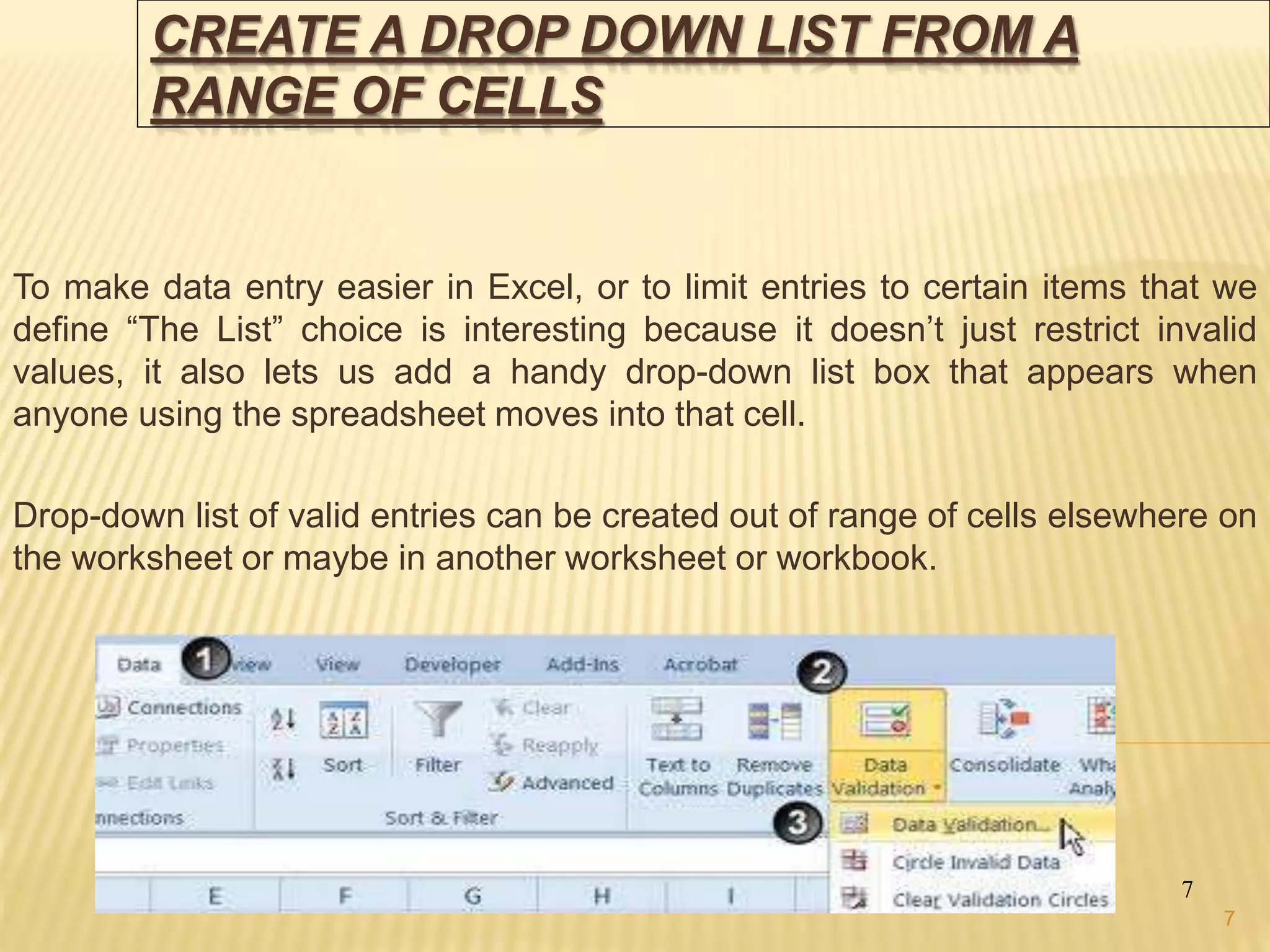
To make data entry easier in Excel, or to limit entries to certain items that we
define “The List” choice is interesting because it doesn’t just restrict invalid
values, it also lets us add a handy drop-down list box that appears when
anyone using the spreadsheet moves into that cell.
Drop-down list of valid entries can be created out of range of cells elsewhere on
the worksheet or maybe in another worksheet or workbook.
7
7

8. APPLY DATA VALIDATION TO CELLS
8
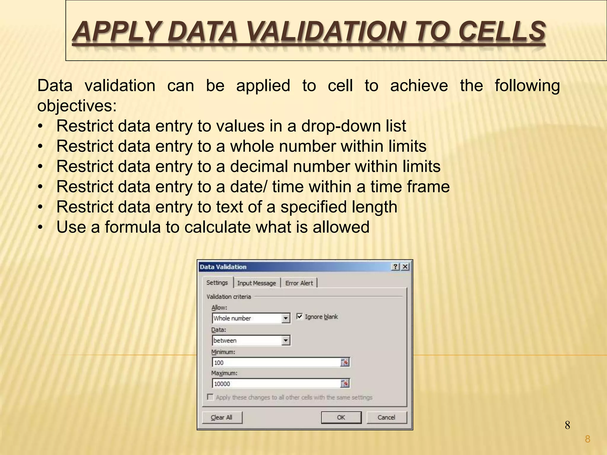
Data validation can be applied to cell to achieve the following
objectives:
• Restrict data entry to values in a drop-down list
• Restrict data entry to a whole number within limits
• Restrict data entry to a decimal number within limits
• Restrict data entry to a date/ time within a time frame
• Restrict data entry to text of a specified length
• Use a formula to calculate what is allowed
8

9. COPY DATA VALIDATION SETTINGS
9
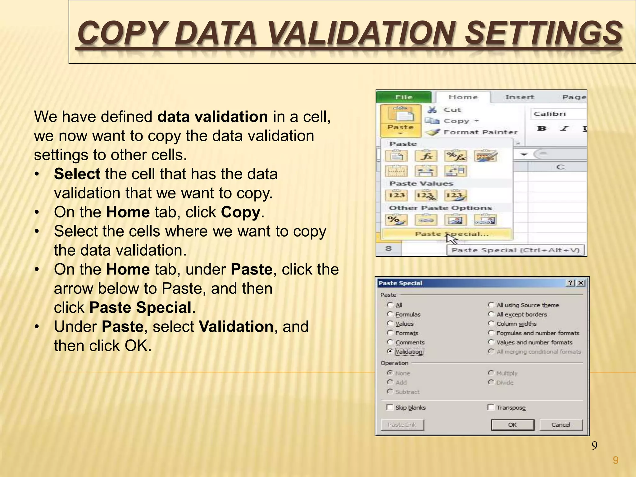
We have defined data validation in a cell,
we now want to copy the data validation
settings to other cells.
• Select the cell that has the data
validation that we want to copy.
• On the Home tab, click Copy.
• Select the cells where we want to copy
the data validation.
• On the Home tab, under Paste, click the
arrow below to Paste, and then
click Paste Special.
• Under Paste, select Validation, and
then click OK.
9

10. FIND CELLS THAT HAVE DATA
VALIDATION
10
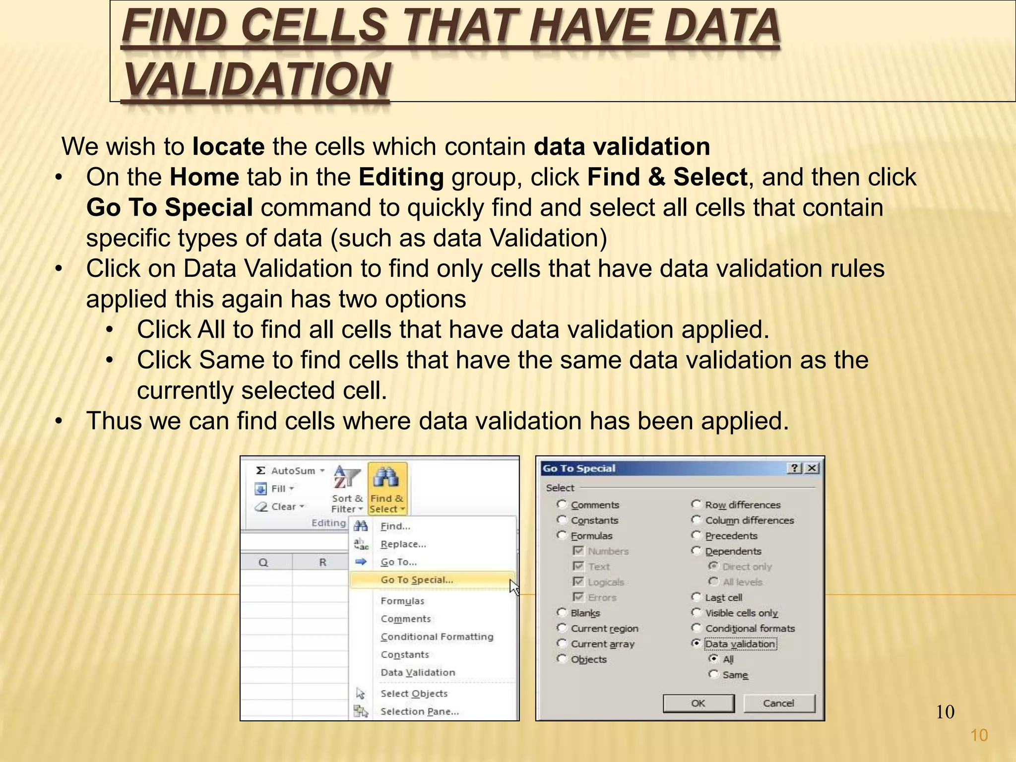
We wish to locate the cells which contain data validation
• On the Home tab in the Editing group, click Find & Select, and then click
Go To Special command to quickly find and select all cells that contain
specific types of data (such as data Validation)
• Click on Data Validation to find only cells that have data validation rules
applied this again has two options
• Click All to find all cells that have data validation applied.
• Click Same to find cells that have the same data validation as the
currently selected cell.
• Thus we can find cells where data validation has been applied.
10

11. USE VALIDATION TO CREATE DEPENDENT
LISTS
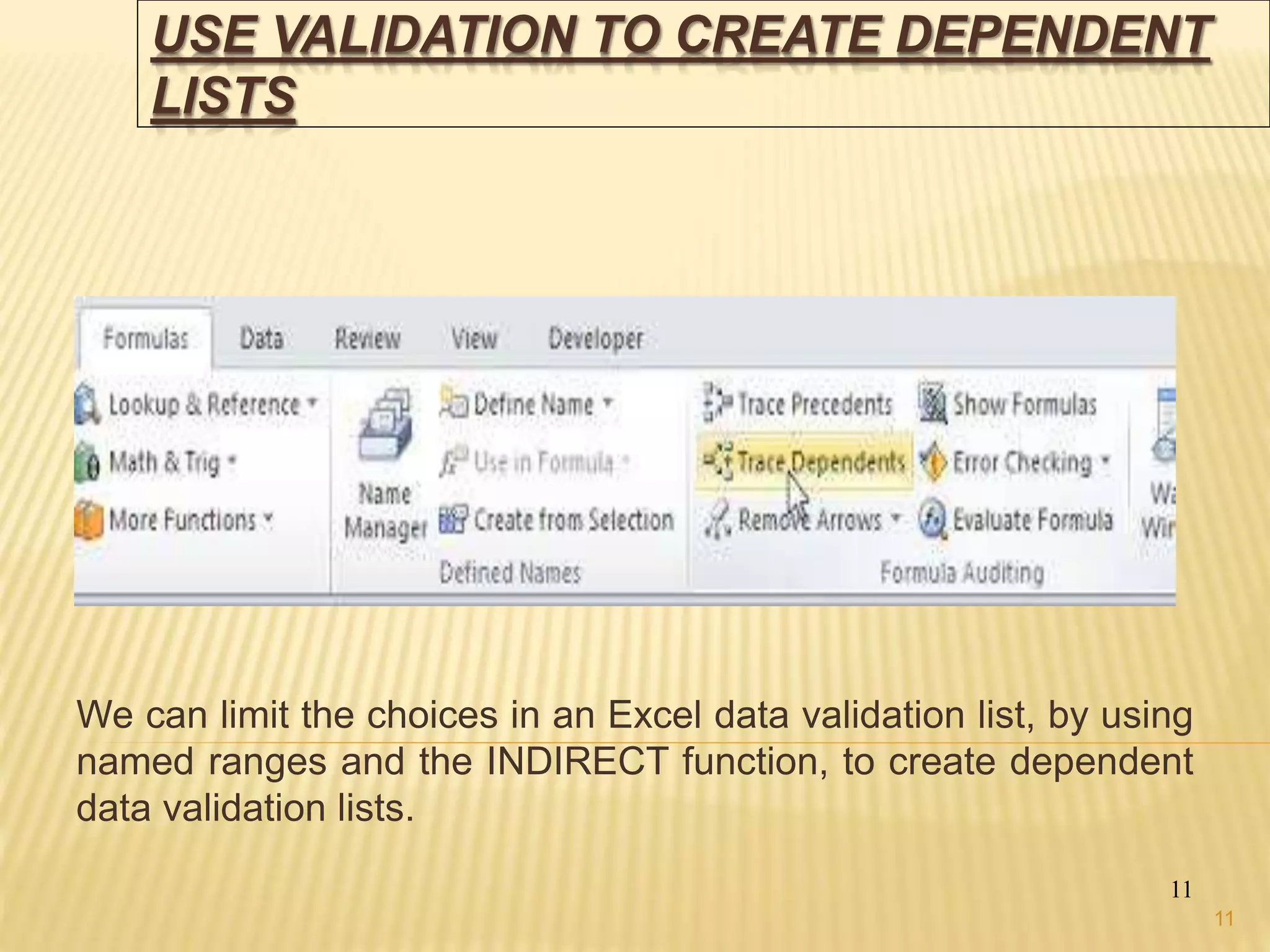
We can limit the choices in an Excel data validation list, by using
named ranges and the INDIRECT function, to create dependent
data validation lists.
11
11

12. DISPLAY OR HIDE CIRCLE AROUND INVALID
DATA
12
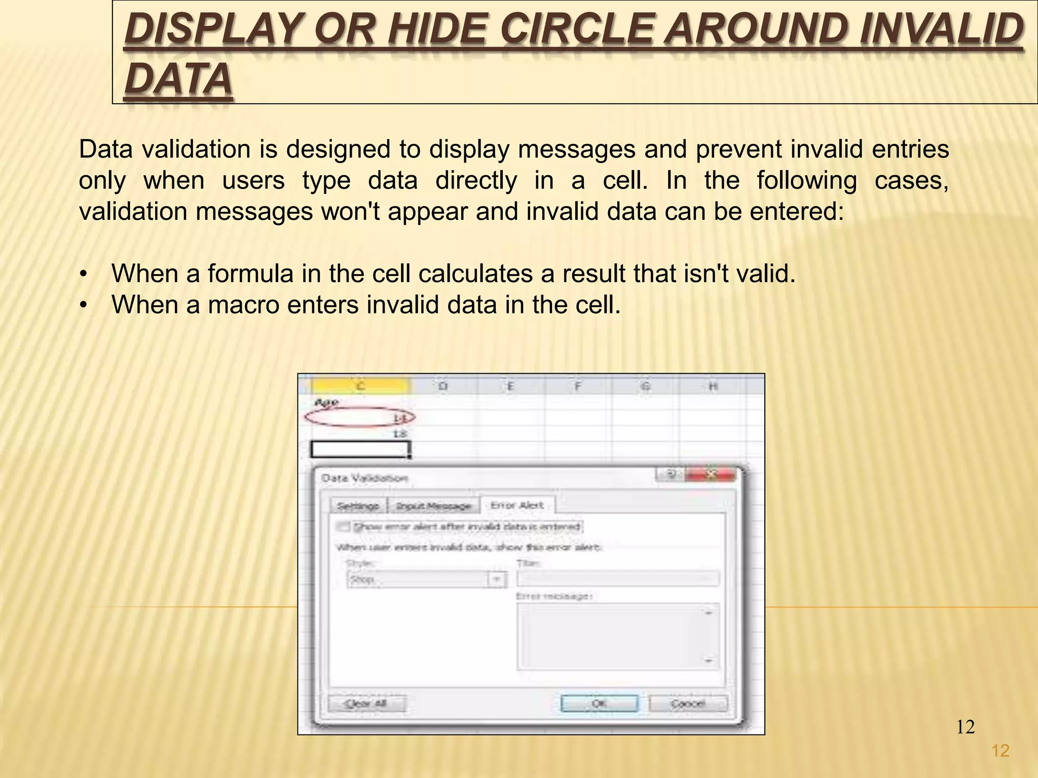
Data validation is designed to display messages and prevent invalid entries
only when users type data directly in a cell. In the following cases,
validation messages won't appear and invalid data can be entered:
• When a formula in the cell calculates a result that isn't valid.
• When a macro enters invalid data in the cell.
12

13. CIRCLE INVALID CELLS
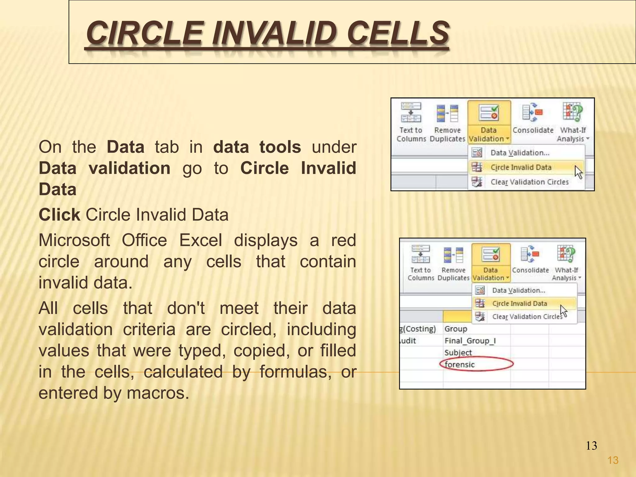
On the Data tab in data tools under
Data validation go to Circle Invalid
Data
Click Circle Invalid Data
Microsoft Office Excel displays a red
circle around any cells that contain
invalid data.
All cells that don't meet their data
validation criteria are circled, including
values that were typed, copied, or filled
in the cells, calculated by formulas, or
entered by macros.
13
13

14. HIDE VALIDATION CIRCLES
14
• We can do one of the following:
• To remove the circle from a single cell, enter valid data in the cell.
• To hide all circles, On the Data tab in data tools under Data
validation go to Clear Invalid Data
14

15. REMOVE DATA VALIDATION
15
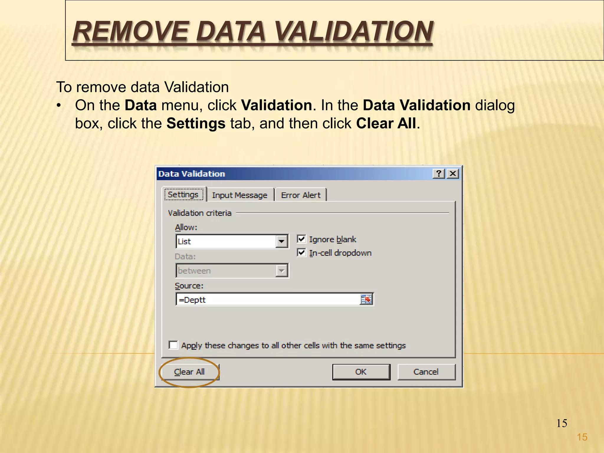
To remove data Validation
• On the Data menu, click Validation. In the Data Validation dialog
box, click the Settings tab, and then click Clear All.
15

16. EXAMPLE -1
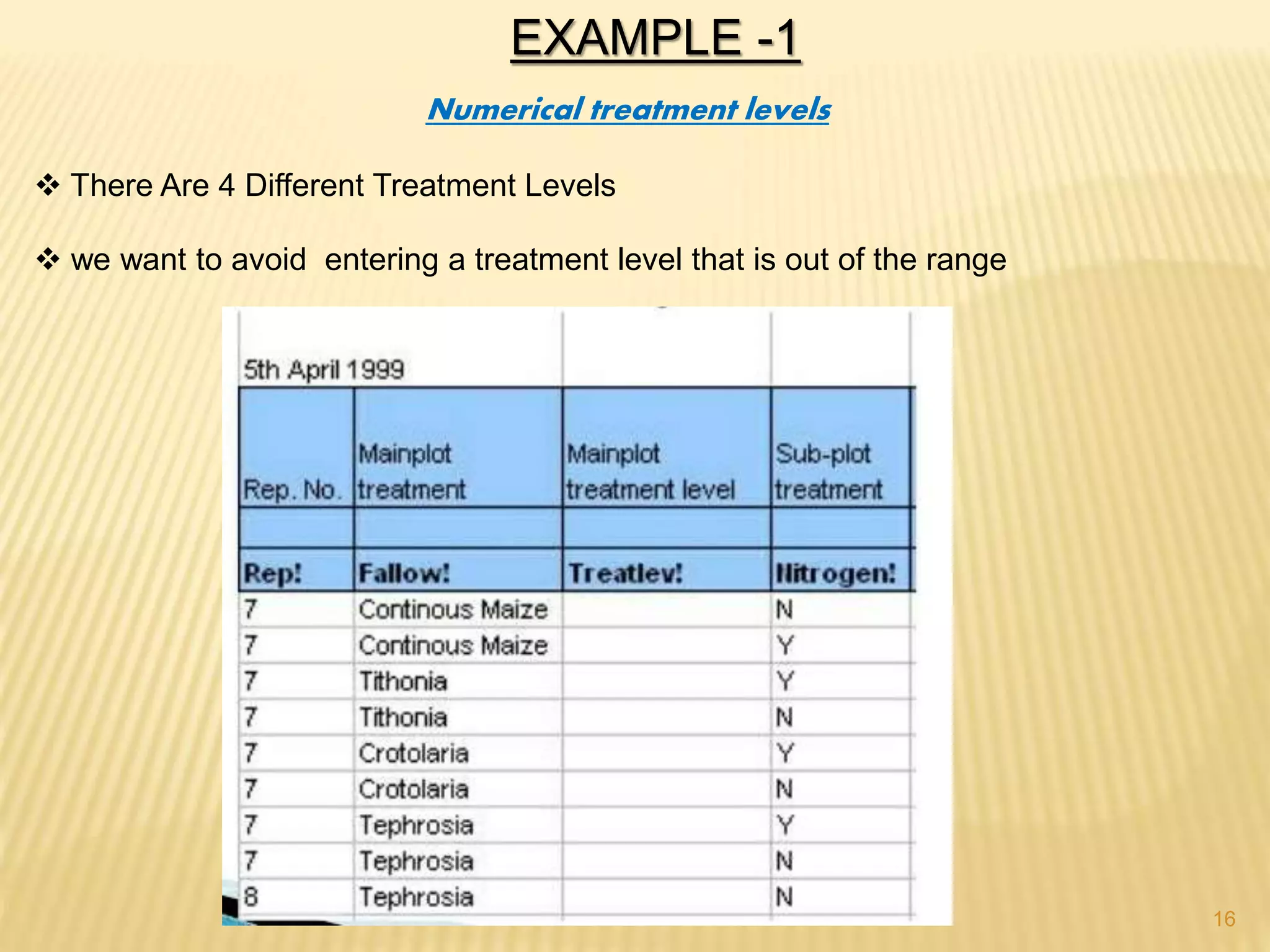
Numerical treatment levels
 There Are 4 Different Treatment Levels
 we want to avoid entering a treatment level that is out of the range
16

17. EXAMPLE -
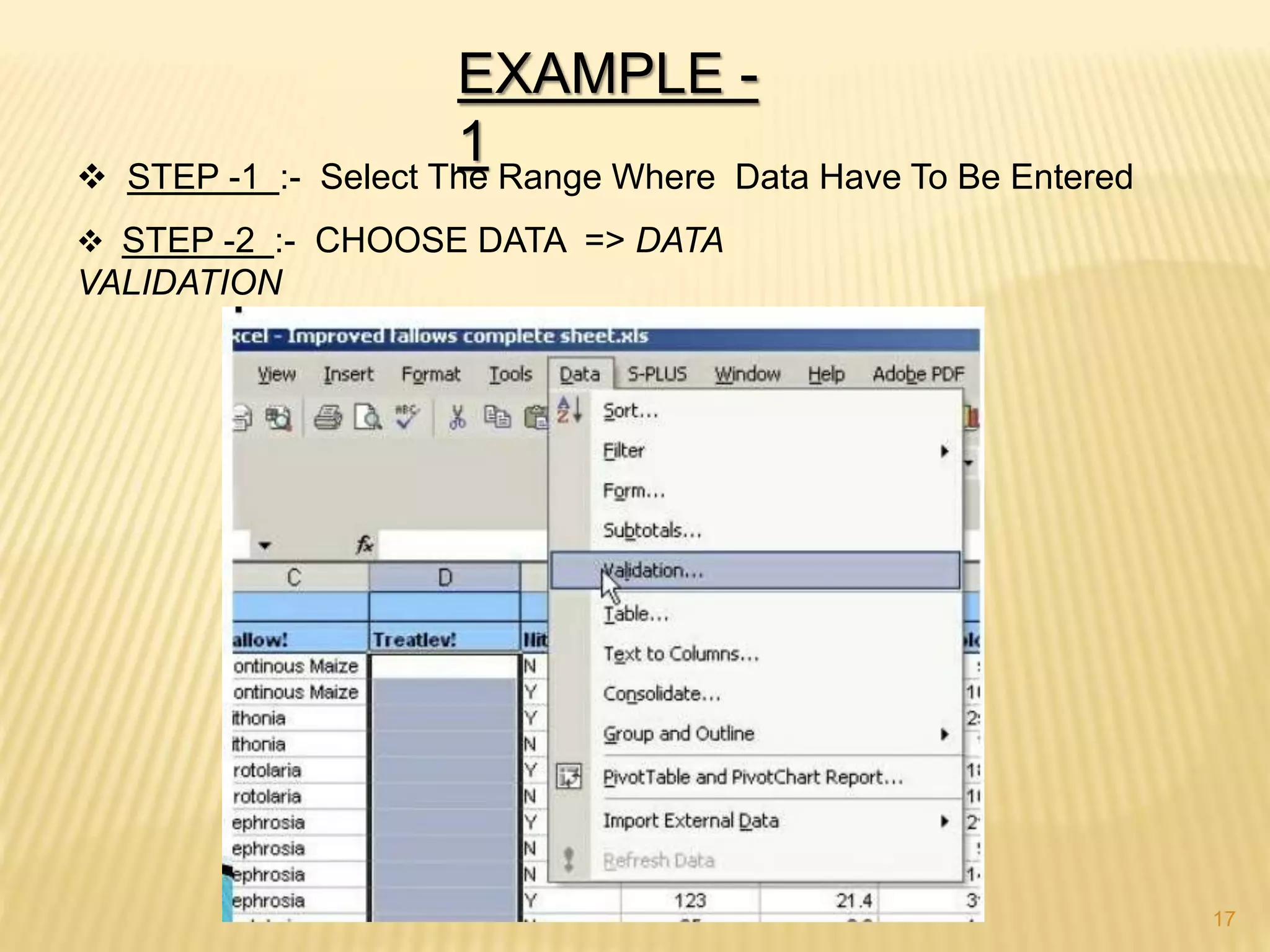
1 STEP -1 :- Select The Range Where Data Have To Be Entered
 STEP -2 :- CHOOSE DATA => DATA
VALIDATION
17

18. EXAMPLE -
1
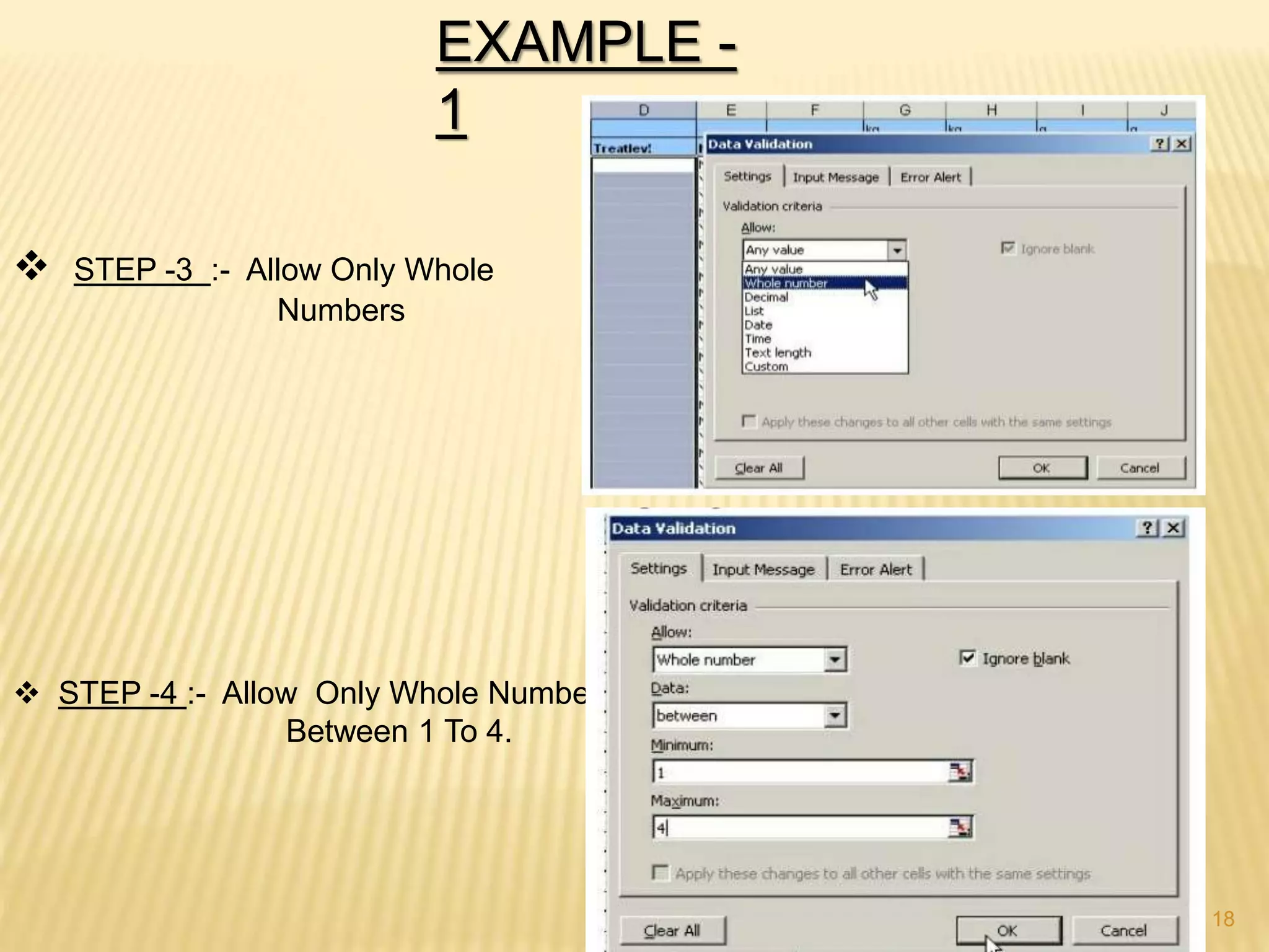
 STEP -3 :- Allow Only Whole
Numbers
 STEP -4 :- Allow Only Whole Numbers
Between 1 To 4.
18

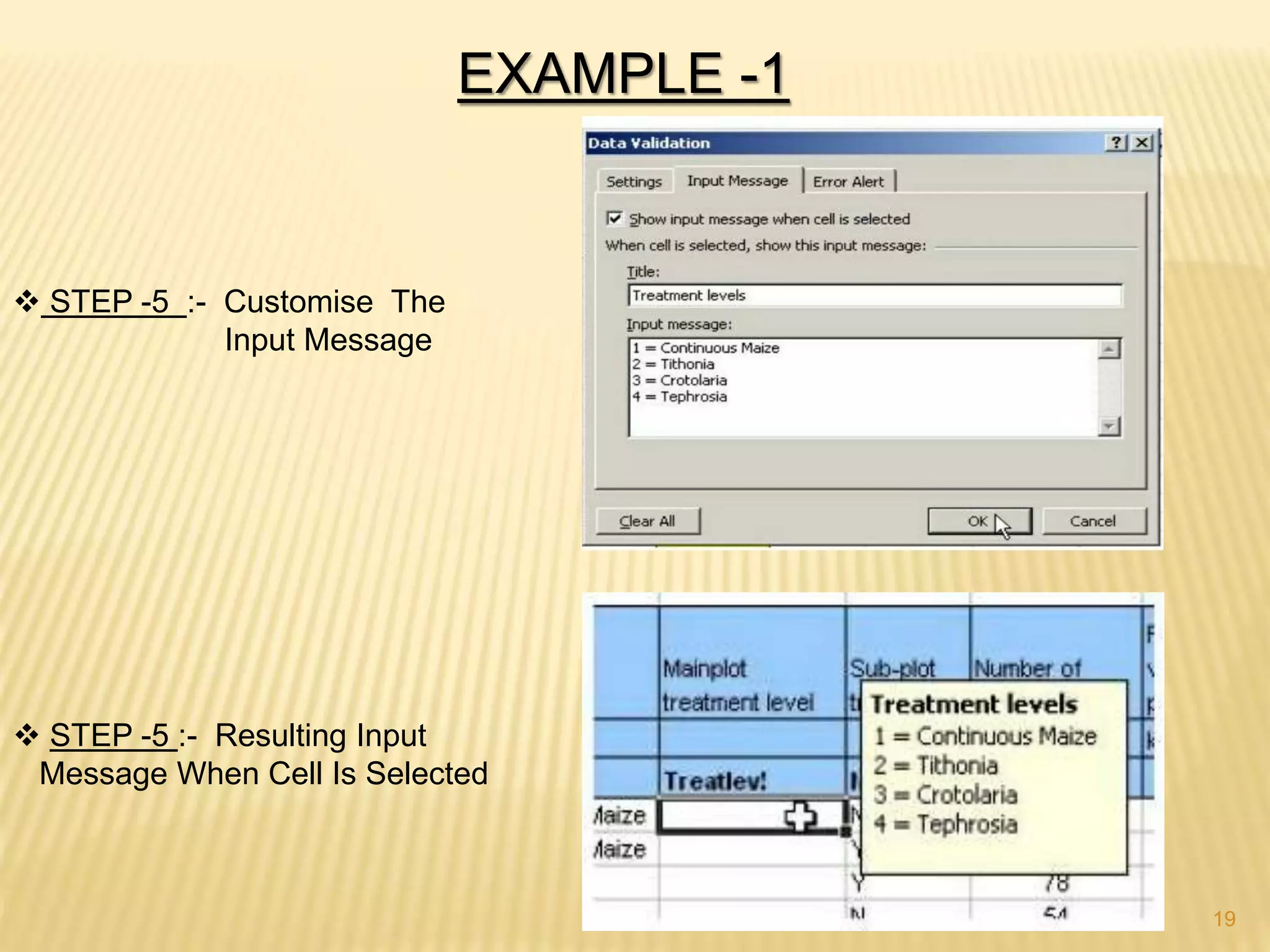
19. EXAMPLE -1
 STEP -5 :- Customise The
Input Message
 STEP -5 :- Resulting Input
Message When Cell Is Selected
19

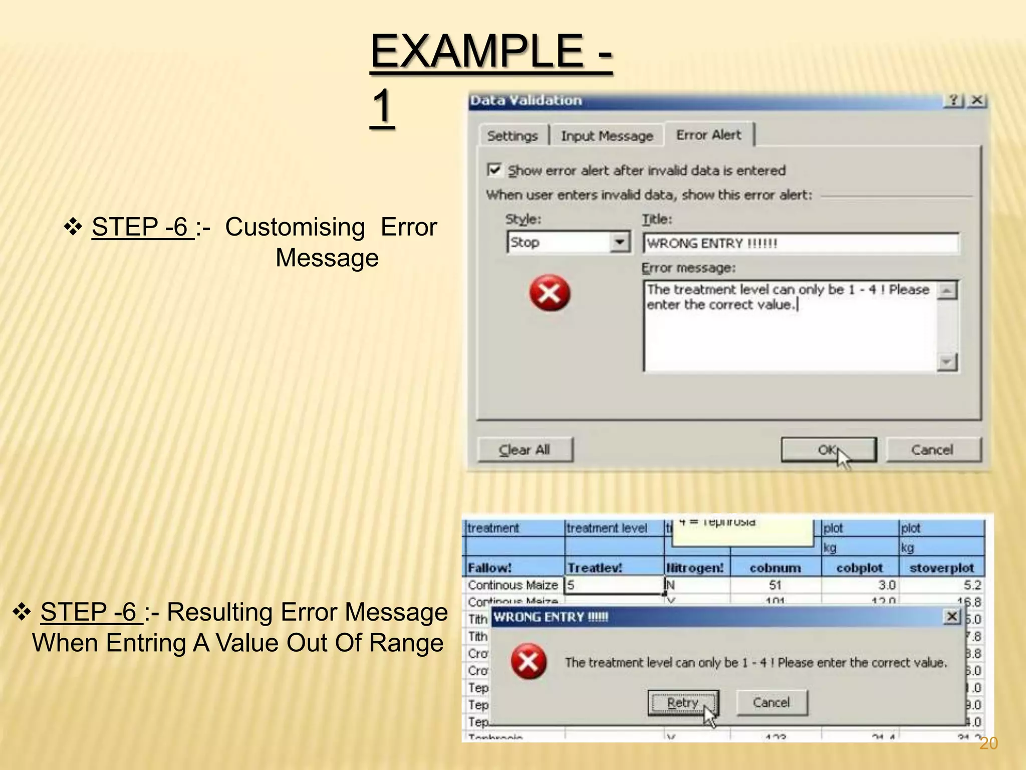
20. EXAMPLE -
1
 STEP -6 :- Customising Error
Message
 STEP -6 :- Resulting Error Message
When Entring A Value Out Of Range
20

21. PART - 2
CONSOLIDATION OF DATA
AND DATAANALYSIS
Microsoft-Excel
21

22. OBJECTIVES
To gain understanding of Working with Tables
To understand Sorting, Filtering, Subtotal
To understand Consolidation of Data
To understand What if Analysis
22
22

23. INTRODUCTION
We enter data into an Excel Worksheet so that we can analyse it,
manipulate it or turn it into a report. So any serious user of excel
should be comfortable working with lists (now Tables in Excel 2010)
organizing data, labeling it, editing it etc.
We can utilize the potential of Excel by putting data in tables.
Each row represents different transaction
Each column represents a different variable ie field
Each column is headed by name of that variable or header.
In the Tables, we might have some preferred order for maintaining
and viewing the records. Depending on the need, we may want the
table arranged alphabetically or date wise as in case of Date of birth
or some custom sort.
23
23

24. SORTING
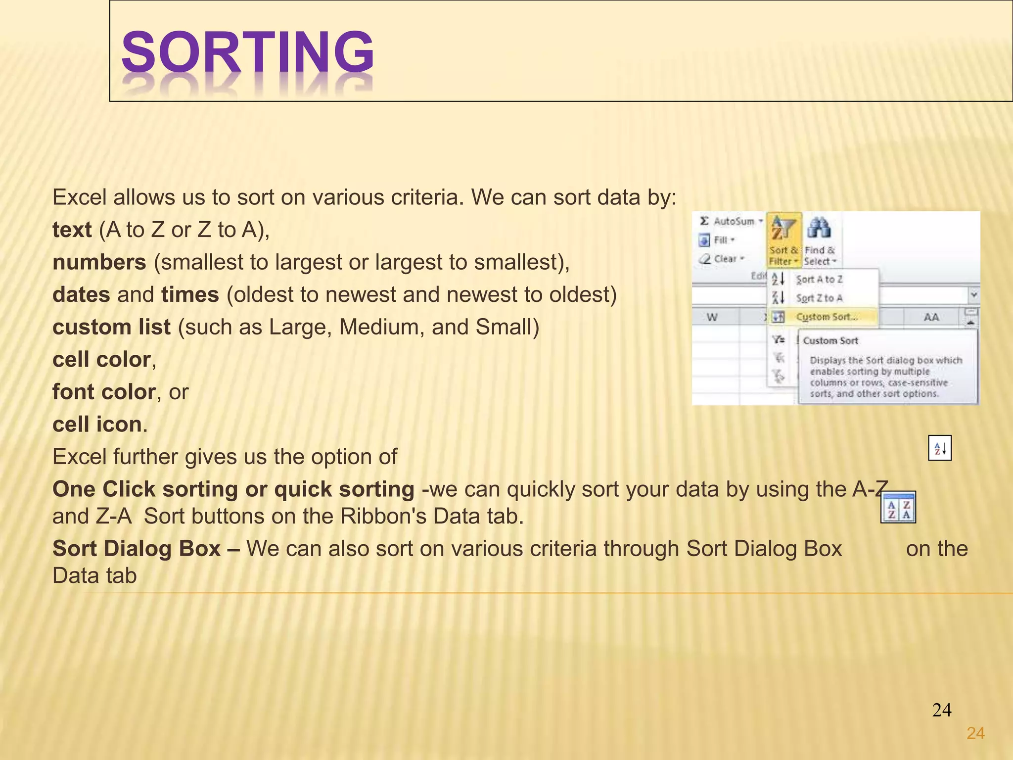
Excel allows us to sort on various criteria. We can sort data by:
text (A to Z or Z to A),
numbers (smallest to largest or largest to smallest),
dates and times (oldest to newest and newest to oldest)
custom list (such as Large, Medium, and Small)
cell color,
font color, or
cell icon.
Excel further gives us the option of
One Click sorting or quick sorting -we can quickly sort your data by using the A-Z
and Z-A Sort buttons on the Ribbon's Data tab.
Sort Dialog Box – We can also sort on various criteria through Sort Dialog Box on the
Data tab
24
24

25. FILTER
25
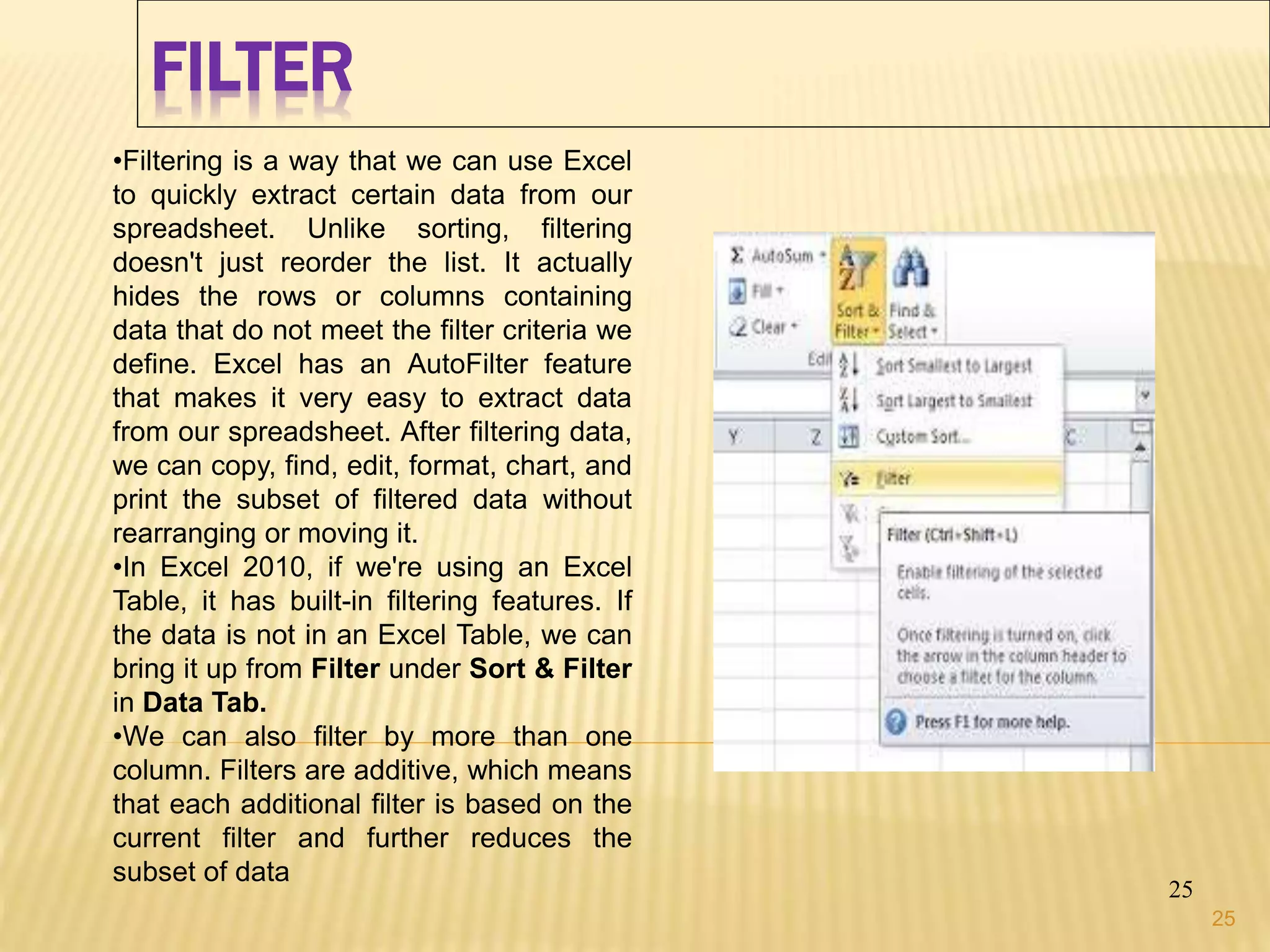
•Filtering is a way that we can use Excel
to quickly extract certain data from our
spreadsheet. Unlike sorting, filtering
doesn't just reorder the list. It actually
hides the rows or columns containing
data that do not meet the filter criteria we
define. Excel has an AutoFilter feature
that makes it very easy to extract data
from our spreadsheet. After filtering data,
we can copy, find, edit, format, chart, and
print the subset of filtered data without
rearranging or moving it.
•In Excel 2010, if we're using an Excel
Table, it has built-in filtering features. If
the data is not in an Excel Table, we can
bring it up from Filter under Sort & Filter
in Data Tab.
•We can also filter by more than one
column. Filters are additive, which means
that each additional filter is based on the
current filter and further reduces the
subset of data
25

26. MORE FILTERING TECHNIQUES
26
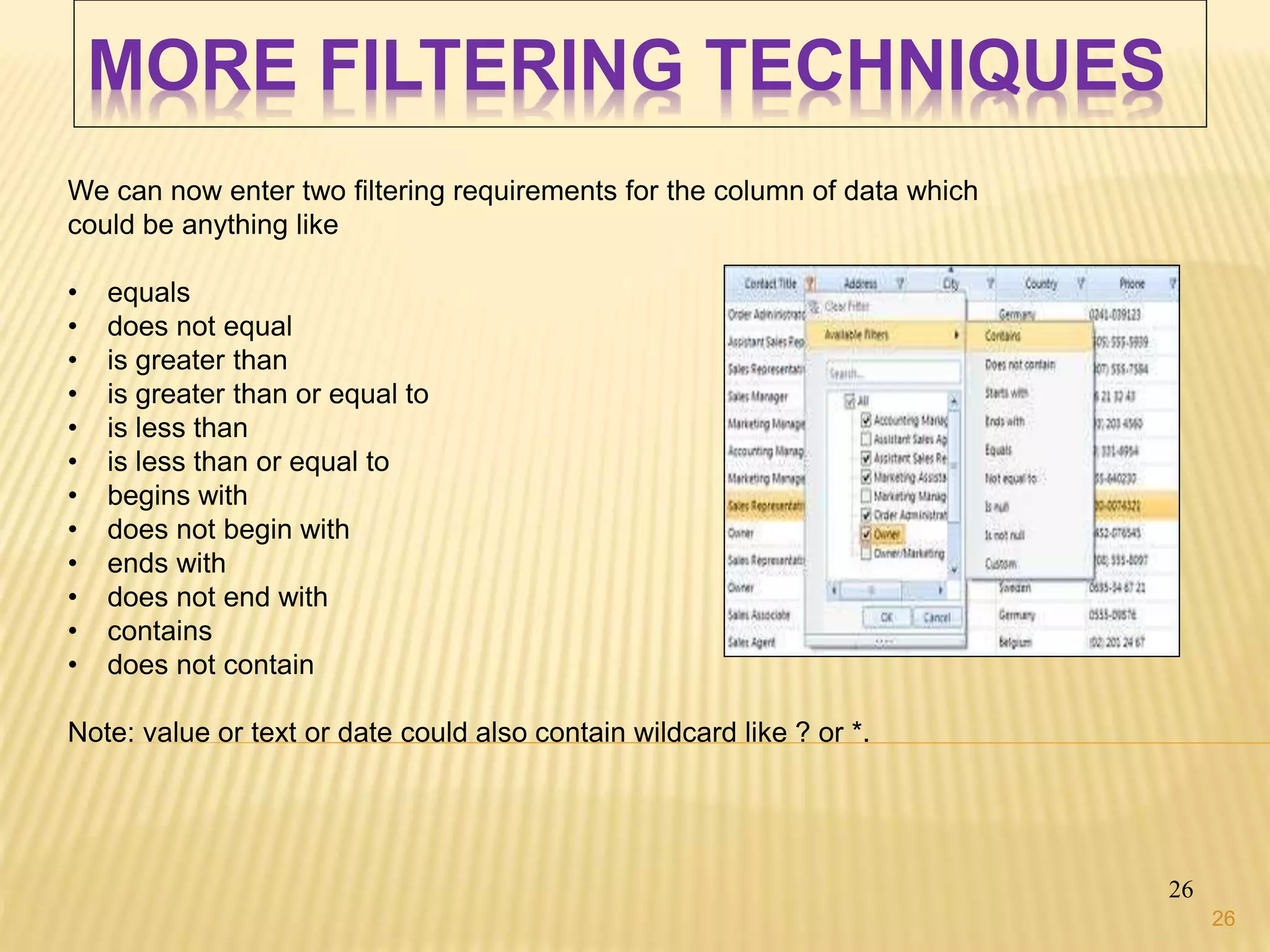
We can now enter two filtering requirements for the column of data which
could be anything like
• equals
• does not equal
• is greater than
• is greater than or equal to
• is less than
• is less than or equal to
• begins with
• does not begin with
• ends with
• does not end with
• contains
• does not contain
Note: value or text or date could also contain wildcard like ? or *.
26

27. SUBTOTALS
27
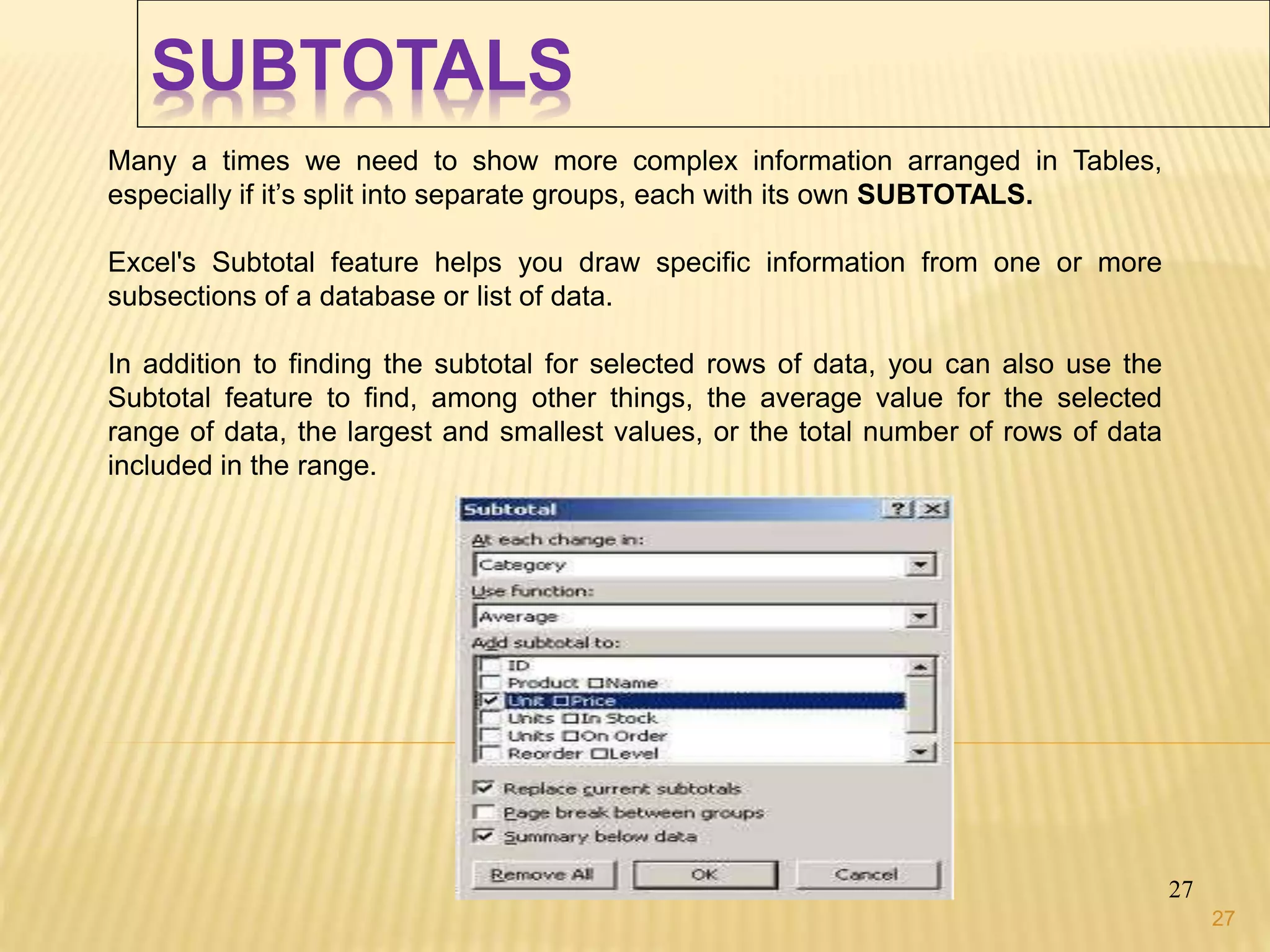
Many a times we need to show more complex information arranged in Tables,
especially if it’s split into separate groups, each with its own SUBTOTALS.
Excel's Subtotal feature helps you draw specific information from one or more
subsections of a database or list of data.
In addition to finding the subtotal for selected rows of data, you can also use the
Subtotal feature to find, among other things, the average value for the selected
range of data, the largest and smallest values, or the total number of rows of data
included in the range.
27

28. CONSOLIDATE
Excel 2010 allows this though CONSOLIDATE feature under Data Tab thereby lets us to
pull-each record from the separate worksheet, consolidating data from into single master
sheet. Consolidation is used for budgets, inventory requirements, business forecasts,
surveys, experimental results and a lot more
Consolidation is the process of combining values from several ranges of data either from
within the same or different workbooks. It can be used to summarize data from different
worksheets into master worksheet and create a report using a variety of calculations
Benefits of consolidation of data:
Easy updating
Aggregation in one window on regular or adhoc basis.
Data can be consolidated in different manner:
Consolidated by Position when all the referring data is in the same location and order,
Consolidate by Category when location and order is not the same.
Consolidated by Formula
Consolidated by Pivot tables
28
28

29. WHAT IF ANALYSIS
29
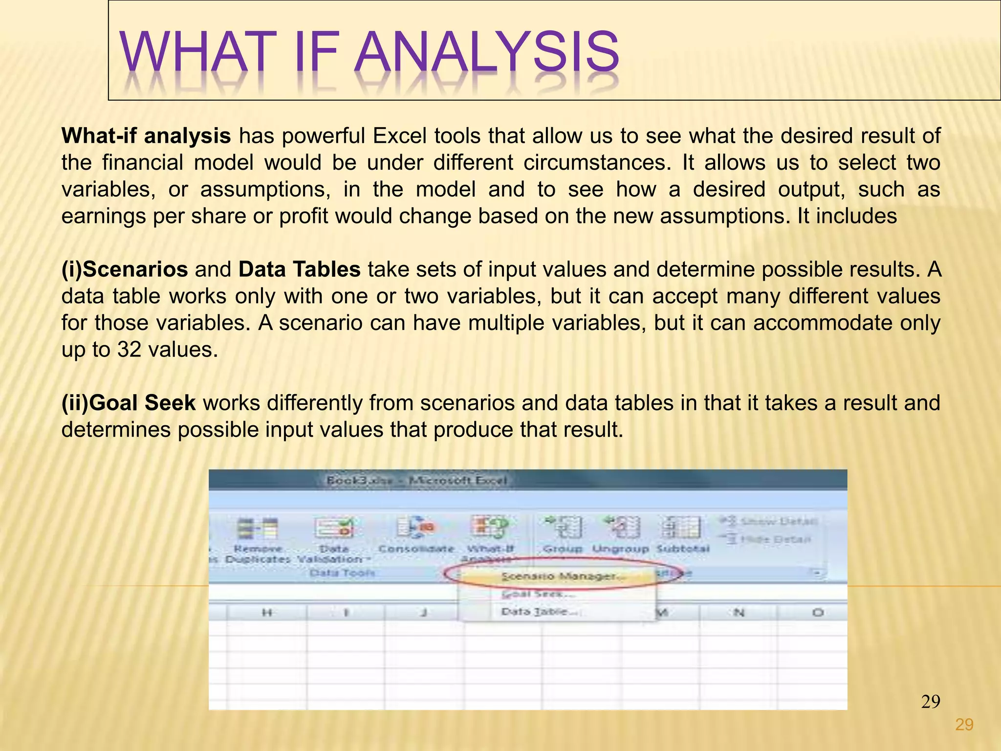
What-if analysis has powerful Excel tools that allow us to see what the desired result of
the financial model would be under different circumstances. It allows us to select two
variables, or assumptions, in the model and to see how a desired output, such as
earnings per share or profit would change based on the new assumptions. It includes
(i)Scenarios and Data Tables take sets of input values and determine possible results. A
data table works only with one or two variables, but it can accept many different values
for those variables. A scenario can have multiple variables, but it can accommodate only
up to 32 values.
(ii)Goal Seek works differently from scenarios and data tables in that it takes a result and
determines possible input values that produce that result.
29

30. 30