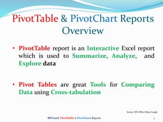
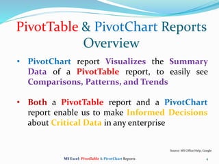
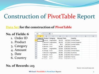
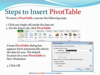
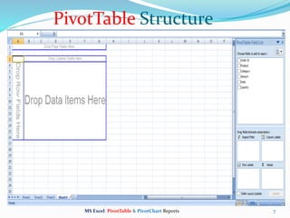
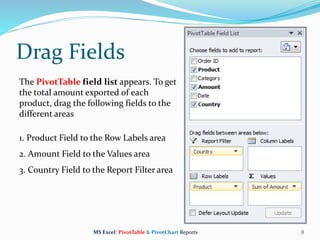
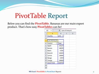
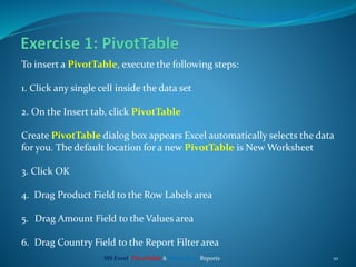
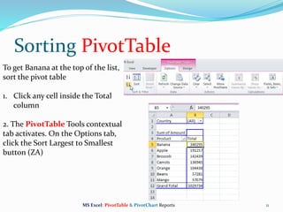
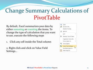
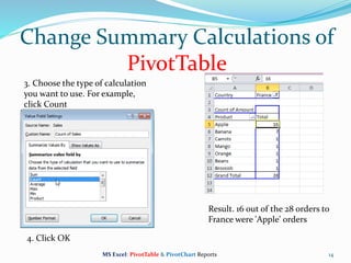
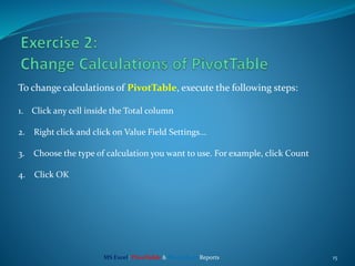
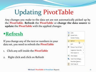
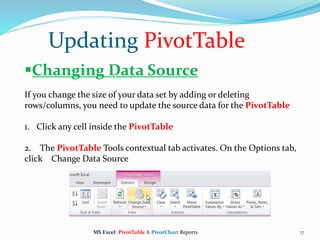
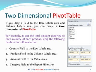
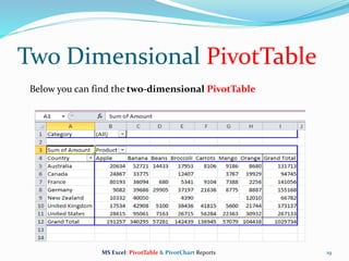
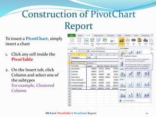
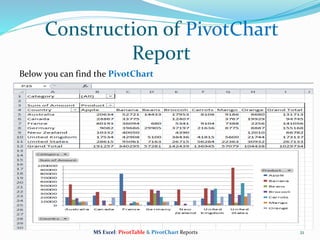
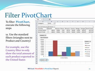
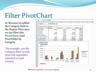
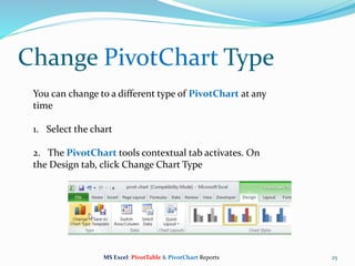
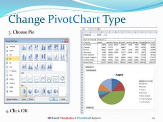
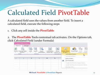
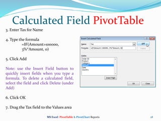
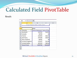
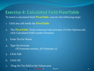
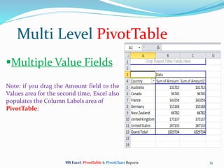
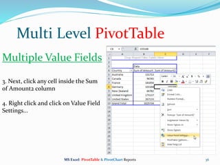
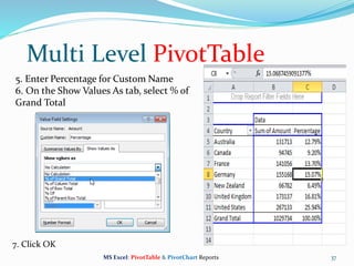
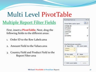
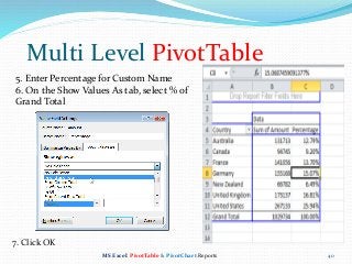
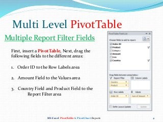
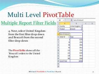
MS Excel Pivot Table Reports & Charts

Word “Pivot” Means
 Spin around
 Spin
 Revolve
 Rotate
 Turn, etc
Source: MS Office online dictionary
2MS Excel: PivotTable & PivotChart Reports

PivotTable & PivotChart Reports
Overview
• PivotTable report is an Interactive Excel report
which is used to Summarize, Analyze, and
Explore data
• Pivot Tables are great Tools for Comparing
Data using Cross-tabulation
3
Source: MS Office Help, Google
MS Excel: PivotTable & PivotChart Reports

PivotTable & PivotChart Reports
Overview
• PivotChart report Visualizes the Summary
Data of a PivotTable report, to easily see
Comparisons, Patterns, and Trends
• Both a PivotTable report and a PivotChart
report enable us to make Informed Decisions
about Critical Data in any enterprise
4
Source: MS Office Help, Google

Construction of PivotTable Report
5
Data Set for the construction of PivotTable
No. of Fields: 6
1. Order ID
2. Product
3. Category
4. Amount
5. Date
6. Country
No. of Records: 213
Source: www.excel-easy.com

Steps to Insert PivotTable
6
To insert a PivotTable, execute the following steps
1. Click any single cell inside the data set
2. On the Insert tab, click PivotTable
Create PivotTable dialog box
appears Excel automatically selects
the data for you. The default
location for a new PivotTable is
New Worksheet
3. Click OK

7
PivotTable Structure

Drag Fields
8
The PivotTable field list appears. To get
the total amount exported of each
product, drag the following fields to the
different areas
1. Product Field to the Row Labels area
2. Amount Field to the Values area
3. Country Field to the Report Filter area

PivotTable Report
9
Below you can find the PivotTable. Bananas are our main export
product. That's how easy PivotTables can be!

10
To insert a PivotTable, execute the following steps:
1. Click any single cell inside the data set
2. On the Insert tab, click PivotTable
Create PivotTable dialog box appears Excel automatically selects the data
for you. The default location for a new PivotTable is New Worksheet
3. Click OK
4. Drag Product Field to the Row Labels area
5. Drag Amount Field to the Values area
6. Drag Country Field to the Report Filter area

Sorting PivotTable
11
To get Banana at the top of the list,
sort the pivot table
1. Click any cell inside the Total
column
2. The PivotTable Tools contextual
tab activates. On the Options tab,
click the Sort Largest to Smallest
button (ZA)

Filter PivotTable
12
Because we added the Country field to
the Report Filter area, we can filter this
PivotTable by Country. For example,
which products do we export the most to
France?
1. Click the filter drop-down and select
France
Result: Apples are our main export
product to France
Note: You can use the standard filter (triangle next to Product) to
only show the totals of specific products

Change Summary Calculations of
PivotTable
13
By default, Excel summarizes your data by
either summing or counting the items. To
change the type of calculation that you want
to use, execute the following steps
1. Click any cell inside the Total column
2. Right click and click on Value Field
Settings...

14
3. Choose the type of calculation
you want to use. For example,
click Count
Result. 16 out of the 28 orders to
France were 'Apple' orders
Change Summary Calculations of
PivotTable
4. Click OK

15
To change calculations of PivotTable, execute the following steps:
1. Click any cell inside the Total column
2. Right click and click on Value Field Settings...
3. Choose the type of calculation you want to use. For example, click Count
4. Click OK

Updating PivotTable
16
Any changes you make to the data set are not automatically picked up by
the PivotTable. Refresh the PivotTable or change the data source to
update the PivotTable with the applied changes
Refresh
If you change any of the text or numbers in your
data set, you need to refresh the PivotTable
1. Click any cell inside the PivotTable
2. Right click and click on Refresh

17
Changing Data Source
If you change the size of your data set by adding or deleting
rows/columns, you need to update the source data for the PivotTable
2. The PivotTable Tools contextual tab activates. On the Options tab,
click Change Data Source
Updating PivotTable

Two Dimensional PivotTable
18
If you drag a field to the Row Labels area and
Column Labels area, you can create a two-
dimensional PivotTable
For example, to get the total amount exported to
each country, of each product, drag the following
fields to the different areas:
1. Country Field to the Row Labels area
2. Product Field to the Column Labels area
4. Category Field to the Report Filter area

19
Below you can find the two-dimensional PivotTable
Two Dimensional PivotTable

Construction of PivotChart
Report
20
To insert a PivotChart, simply
insert a chart
1. Click any cell inside the
PivotTable
2. On the Insert tab, click
Column and select one of
the subtypes
For example, Clustered
Column

21
Below you can find the PivotChart
Construction of PivotChart
Report

22
To insert a PivotChart, execute the following steps:
2. On the Insert tab, click Column and select one of the subtypes
For example, Clustered Column

Filter PivotChart
23
To filter PivotChart,
execute the following
steps
1a. Use the standard
filters (triangles next to
Product and Country)
For example, use the
Country filter to only
show the total amount of
each product exported to
the United States

24
1b. Because we added
the Category field to
the Report Filter area,
we can filter this
PivotChart (and
PivotTable) by
Category
For example, use the
Category filter to only
show the vegetables
exported to each
country
Filter PivotChart

Change PivotChart Type
25
You can change to a different type of PivotChart at any
time
1. Select the chart
2. The PivotChart tools contextual tab activates. On
the Design tab, click Change Chart Type

26
3. Choose Pie
Change PivotChart Type
4. Click OK

Calculated Field PivotTable
27
A calculated field uses the values from another field. To insert a
calculated field, execute the following steps
click Calculated Field (under Formula)

28
3. Enter Tax for Name
4. Type the formula
=IF(Amount>100000,
3%*Amount, 0)
5. Click Add
Note: use the Insert Field button to
quickly insert fields when you type a
formula. To delete a calculated field,
select the field and click Delete (under
Add)
6. Click OK
7. Drag the Tax field to the Values area

29
Result:

30
To insert a calculated field PivotTable, execute the following steps:
click Calculated Field (under Formula)
3. Enter Tax for Name
4. Type the formula
=IF(Amount>100000, 3%*Amount, 0)
5. Click Add
6. Click OK
7. Drag the Tax field to the Values area

Multi Level PivotTable
31
It's perfectly ok to drag more than one field to an area in a
PivotTable. We will look at an example of Multiple Row Fields,
Multiple Value Fields and Multiple Report Filter Fields
Data Set for Multi Level PivotTable
No. of Fields: 6
1. Order ID
2. Product
3. Category
4. Amount
5. Date
6. Country
No. of Records: 213

32
First, Insert a PivotTable, Next, drag the
following fields to the different areas:
1. Category Field and Country Field to the
Row Labels area
Multiple Row Fields

33
Multiple Row Fields

34
First, insert a PivotTable, Next, drag the
1. Country Field to the Row Labels area
2. Amount Field to the Values area (2x)
Multiple Value Fields

35
Multiple Value Fields
Note: if you drag the Amount field to the
Values area for the second time, Excel also
populates the Column Labels area of
PivotTable:

36
3. Next, click any cell inside the Sum
of Amount2 column
4. Right click and click on Value Field
Settings...
Multiple Value Fields

37
5. Enter Percentage for Custom Name
6. On the Show Values As tab, select % of
Grand Total
7. Click OK

38
First, insert a PivotTable, Next, drag the
1. Order ID to the Row Labels area
3. Country Field and Product Field to the
Report Filter area
Multiple Report Filter Fields

39
4. Next, select United Kingdom
from the first filter drop-down
and Broccoli from the second
filter drop-down
Multiple Report Filter Fields
The PivotTable shows all the
'Broccoli' orders to the United
Kingdom

MS Excel Pivot Table Reports & Charts

MS Excel Pivot Table Reports & Charts

More Related Content

What's hot

Viewers also liked

Similar to MS Excel Pivot Table Reports & Charts

Recently uploaded

MS Excel Pivot Table Reports & Charts