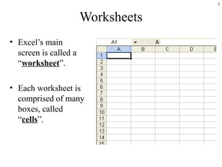
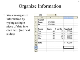
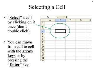
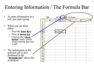
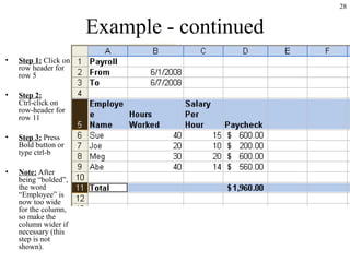
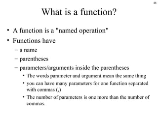
SlideShare a Scribd company logo
1 of 164
1
Introduction to
Excel
Yitzchak Rosenthal
Worksheet
Basics
2
3
Worksheets
• Excel’s main
screen is called a
“worksheet”.
• Each worksheet is
comprised of many
boxes, called
“cells”.
4
Organize Information
• You can organize
information by
typing a single
piece of data into
each cell. (see next
slides)
5
How to Enter Information
6
Selecting a Cell
• “Select” a cell
by clicking on it
once (don’t
double click).
• You can move
from cell to cell
with the arrow
keys or by
pressing the
“Enter” key.
7
Entering Information / The Formula Bar
• To enter information in a
cell, just start typing.
• When you are done
either
– Press the Enter Key
– Press an arrow key
– Click on the “check
button” (only visible
when entering data into
a cell)
• The information in the
selected cell is also
displayed in the
“formula bar” above the
worksheet.
8
Double Click to Modify a Cell
• To modify the contents
of a cell double click
on the cell.
• Then use the right, left
arrow keys and the
Insert and Delete keys
to modify the data.
• When you are done:
– Press the Enter key
or
– Click on the check box.
Double click to
change “hi there” to
“hello there”
9
Names of Rows, Columns and
Cells
10
Column Names (letters) & Row Names (numbers)
• The columns of
the worksheet
are named with
letters
• The rows are
named with
numbers
Selected
Cell
11
Cell Names (ex. B4)
• The name of a cell is a combination
of the Letter Of The Column that
the cell is in followed by the
Number Of The Row that the cell is
in.
• Example: the selected cell in the
picture is named B4 (NOT 4B)
• Excel automatically shows the the
name of the currently selected cell
in the “name box” (located above
the worksheet).
• The letter must come first (i.e. B4,
NOT 4B) and there may NOT be any
spaces between the letter and the
number.
• We will learn later why it is
important to understand how to name
cells.
Name
Box
Selected
Cell
12
Longggggggg Data
13
Information that is “too wide” for a cell
• The word “Name” is in cell
A5
• The words “Hours Worked”
are in cell B5 (NOT in cell
C5). However, since the
information is too wide for
cell B5, it looks like it
extends into cell C5.
• You can determine that the
information is really only IN
cell B5 by selecting cell B5
and looking at the formula
bar and then selecting cell
C5 and looking at the
formula bar.
“Hours
Worked” is
in cell B5
(look at
formula bar)
“Hours
Worked” is
NOT in cell
C5 (formula
bar is empty)
14
Information that is “Chopped Off”
• If there is information
in the cell to the right,
then the original cell
still contains all of the
data, but the data
appears to be
“chopped off”.
• You can see the
complete data by
selecting the cell and
looking in the
formula bar.
15
Change the Width of a Column or
the Height of a Row
16
Make a column wider
• To make Column B wider,
point the cursor to the
column separator between
columns B and column C.
• The cursor changes to a
“Double headed arrow”.
• Now, click the left mouse
button and without letting
go of the button, drag the
separator to the right to
make the column wider (or
to the left to make the column
narrower).
Column is now wider
Drag column
separator to the
right
17
Getting the Exact Width
• To get the “exact” width,
double click on the
separator instead of
dragging it.
Column is now EXACTLY the correct width
Double click here
18
Resizing a Row
• Make a row
taller or
shorter by
dragging
the
separator
between the
rows.
• Click and
drag here to
resize row
5.
Row is now
taller
19
Putting an “Enter” inside a cell
• To add a new line
inside a cell
– Double click inside
the cell where you
want the new line.
– Press Ctrl-Enter
(i.e. hold down the
Ctrl key and press
Enter while still
holding down
Ctrl).
– When you are done
editing, press Enter
(without holding
down Ctrl) to
accept the changes.
Step 1: Originally
“Hours Worked”
is on one line.
Step 2: Double click
to edit cell and then
press Ctrl-Enter
Step 3: Press Enter
(without Ctrl) to
accept the changes.
20
Basic Formatting
(e.g. bold, colors, fonts, etc)
21
Formatting Cells
• Select one or more cells and then click on any of the formatting buttons (see
below) to change the formatting of the selected cells.
• Formatting buttons:
font
name
font
size
bold
italics
underline
center & merge
cells
(will explain later)
center
right justifyleft justify
These change the way
numbers are displayed
in cells. (these don’t
affect words).
show as currency
(ex. 1000.507 becomes $1000.50)
show with commas (e.g.
12345 becomes 12,345)
show as percent (ex.
0.5 becomes 50%)
remove indent
show fewer decimal points (ex.
10.507 is displayed as 10.51)
show more decimal points (ex.
10.507 is displayed as 10.5070)
indent within cell
put border around cell(s)
color of cell
color of
text in cell
click on
downward
pointing arrows
for other colors
and border
styles
click on
downward
pointing arrows
for other font
names and
sizes
22
Example – unformatted worksheet
• Unformatted worksheet – see next slide for formatting.
23
Example –making cells bold
• Click on cell A1 and drag to cell A3.
• Then press the Bold button to make cells A1,A2,A3 bold.
• You could also press the font or background color buttons to change the color
or apply any other formatting you like (this is not shown below).
24
Other Ways of Selecting More Than One
Cell
• To select a large range of cells, click on the upper
left cell in the range. Then hold the shift key and
click on the lower right cell in the range.
• You can select different “non-contiguous” areas of
cells by holding down the Ctrl key while clicking
and dragging.
25
Selecting Non-Contiguous Ranges
• Click and
drag to
select the
first
range.
• Ctrl-click
and drag
to select
additional
ranges
(This cell is also selected
even though it appears
white).
26
Selecting entire Rows, entire Columns or
all cells on the worksheet.
• To select an entire column, click on the letter for
the column header. To select several columns,
click on the header for the first column and drag to
the right.
• To select an entire row, click on the number for the
row header. To select several rows, click on the
header for the first row and drag down.
• To select all of the cells on the spreadsheet, click
on the upper left hand corner of the spreadsheet
(where the column headers meet the row headers)
27
Select Entire Columns/Rows/Worksheet
To select ENTIRE COLUMN B
click on “B” column header
To select COLUMNS B,C,D
click on “B” column header and drag to right
To select COLUMNS B,C and F,G,H
– click on “B” column header, drag to right,
– then Ctrl-Click on “F” column header and drag right
To select ENTIRE ROW 2
click on “2” row header
To select ROWS 2,3 and 5,6,7
– click on “2” row header, drag down,
– then Ctrl-Click on “5” row header and drag down
To select ENTIRE WORKSHEET
click on select worksheet button
(in corner between “1” and “A” buttons)
ClickClick
drag
Click
drag
Click and drag down
then Ctrl-Click
and drag down
Clickdrag
Ctrl-
Click
Click
28
Example - continued
• Step 1: Click on
row header for
row 5
• Step 2:
Ctrl-click on
row-header for
row 11
• Step 3: Press
Bold button or
type ctrl-b
• Note: After
being “bolded”,
the word
“Employee” is
now too wide
for the column,
so make the
column wider if
necessary (this
step is not
shown).
29
More Advanced Formatting
30
Format Cells
• Using the formatting buttons only
give you a limited amount of
formatting ability.
• For more formatting ability, select
one or more cells and right click on
the selection. Then choose “format
cells” from the popup menu.
• Choose options from the Number,
Alignment, Font, Border and
Patterns tabs and press OK to
change the way your information
looks on the screen.
• The Protection tab is used to lock
cells so that their contents can’t be
modified.
• We will not go into the details of
using the format cells dialog box at
this time but you should be able to
figure out most of it by yourself.
31
Formatting changes how things LOOK,
not how they WORK.
• NOTE: you will probably not understand this slide
until after you learn about Excel Formulas.
Formulas are covered later in this presentation.
• When you change the format of a cell, Excel still
“remembers” the original value.
• Excel will use the un-formatted value when
calculating formula values.
• Example: if you change numbers to appear with
fewer decimal points the original number with all
of its decimal points are used in calculations.
Formulas
The bread and butter of Excel
32
33
Excel Formulas
• You must have an equals sign ( = ) as the first
character in a cell that contains a formula.
• The = sign tells excel that the contents of the cell
is a formula
• Without the = sign, the formula will not calculate
anything. It will simply display the text of the
formula.
34
Formulas - correct
formula with = sign After pressing ENTER
35
Missing = sign
Missing = sign!
Before pressing enter
After pressing ENTER
(no change - not a function)
36
Types of operations
• You can use any of the following operations in a
formula:
operation symbol example
addition: + =a1+3
subtraction: - =100-b3
multiplication: * =a1*b1
division: / =d1/100
exponentiation ^ =a2^2
negation - =-a2+3
(same symbol as subraction)
37
Explicit (literal) values and cell references
• You can use both explicit values and cell
references in a formula
• An explicit value is also called a literal value
– Formula with only cell references: =a1*b1
– Formula with only literal values: =100/27
– Formula with both cell references and literal values:
=a1/100
38
Errors in Formulas
39
Common Errors
• The following are some errors that may appear in a spreadsheet (there are others too).
– #######
• Cell is too narrow to display the results of the formula. To fix this simply make the column wider and
the “real” value will be displayed instead of the ###### signs. Note that even when the ###### signs are
being displayed, Excel still uses the “real” value to calculate formulas that reference this cell.
– #NAME?
• You used a cell reference in the formula that is not formed correctly (e.g. =BB+10 instead of =B3+10)
– #VALUE!
• Usually the result of trying to do math with a textual value. Example: =A1*3 where A1 contains the
word “hello”
– #DIV/0!
• Trying to divide by zero. Example: =3/A1 where A1 contains 0 (zero)
– Circular Reference
• Using a formula that contains a reference to the cell that the formula “lives in”. Example: putting the
formula =A1+1 in cell A1 or putting the formula =SUM(A1:B2) in any of the cells A1, B1, A2, B2
40
Order of Operations
41
Complex formulas
• You can use several operations in one function
• You can group those operations with parentheses
• Examples
=3*2+1
=c1*(a1+b1)
=(100*a2-10)+(200*b3-20)+30
=(3+2*(50/b3+3)/7)*(3+b7)
42
Order of operations
• When using several operations in one formula,
Excel follows the order of operations for math.
– first: all parentheses - innermost first
– second: exponents (^)
– third: all multiplication (*) and division (/). Do
these starting with the leftmost * or /
and work to the right.
– fourth: all addition (+) and subtraction (-). Do
these starting with the leftmost + or -
and work to the right.
43
Please Excuse My Dear Aunt Sally
• The sentence "Please excuse my dear aunt Sally" is a
popular mneumonic to remember the order of operations:
Menumonic Meaning
– Please parentheses
– Excuse exponents
– My Dear mulitplication and division
(going left to right)
– Aunt Sally addition and subtraction
(going left to right)
44
Order of operations
• The value of
3 + 2 * 5
is
13
NOT 25!
45
Order of operations
3 + (100 - 20) / 10 - 6 * 2 / 4 + 9
3 + 80 / 10 - 6 * 2 / 4 + 9
3 + 8 - 6 * 2 / 4 + 9
3 + 8 - 12 / 4 + 9
3 + 8 - 3 + 9
11 - 3 + 9
8 + 9
answer: 17
46
Cntrl-`
• To see the formulas in the worksheet
– Press the Cntrl key at the same time as you press the `
key (i.e. Cntrl-`)
– Press Cntrl-` again to see the values
47
Functions
48
What is a function?
• A function is a "named operation"
• Functions have
– a name
– parentheses
– parameters/arguments inside the parentheses
• The words parameter and argument mean the same thing
• you can have many parameters for one function separated
with commas (,)
• The number of parameters is one more than the number of
commas.
49
The SUM function
• Examples
Function Result
=SUM(1,2,3,4,5) 15
=SUM(a1,b1,c1) a1+b1+c1
=SUM(9,a1,b2,5,c1) 9+a1+b2+5+c1
50
Terminology
SUM(1,2,3,4,5)
– The name of the function is "SUM"
– The parameters or arguments to this function are
1,2,3,4 and 5
– The entire thing, i.e. SUM(1,2,3,4,5), is a function call
– The value of this function call is 15.
Another way to say this is that this function call
returns 15.
Ranges (e.g. a1:c3)
51
Ranges
• A rectangular box of cells is called a “range”.
• The name of a range is
– the name of the upper left cell of the range
– Followed by a colon :
– Followed by the lower right cell of the range
• Example: A1:B2 is shorthand for A1,A2,B1,B2
– See next slide for more examples
52
A1:B2
Examples of Range Names
• Examples
C3:E10
B2:B5
B3:E3
53
54
Using a range as a parameter
• Ranges can be specified as a parameters to a function call.
• Both of the following function calls produce the same
result as =a1+b1+c1+a2+b2+c2+a3+b3+c3+a4+b4+c4
however the 2nd
version uses a range and is much shorter.
without a range
=SUM(a1,b1,c1,a2,b2,c2,a3,b3,c3,a4,b4,c4)
with a range
=SUM(a1:c4)
55
Function calls with multiple parameters
• You can include multiple ranges and cells as parameters
• Example: the following function call has 3 parameters.
There are two ranges (a1:b2 and c4:c7), one number (100)
and one cell reference (d3)
=SUM(a1:b2,100,c4:c7,d3)
Is the same as:
=SUM(a1,a2,b1,b2,100,c4,c5,c6,c7,d3)
Other Functions
56
57
Other functions
• Click the function button to see the available
functions:
Function buton
brings up the
function dialog box
(see next slide)
58
Function dialog box
categories
(i.e. groups of functions)
Functions for the selected category
Description
of currently
selected
function
Warning: this slide was created using
Excel 2000. The dialog box in later
versions of Excel looks a little different,
but it has the same functionality.
59
Function Editor
• Double click on the function name to get a dialog
box that helps you enter values for the parameters
of the function.
(see next slide)
60
Function Editor
When you press OK, this will create
the function call:
AVERAGE(2,a1:c2,f13)
Put values for the parameters in
the edit boxes.
61
Example
• AVERAGE
formula that contains a function value
=AVERAGE(2,4,10,4) 5
=AVERAGE(a1,f32) (a1+f32) / 2
=AVERAGE(a1:c1) (a1+b1+c1) / 3
=AVERAGE(a1:c1,10) (a1+b1+c1+10) / 4
62
Combining Functions and other values
in a single formula
63
Functions and other values
• You can combine functions, cell references and
literal values to make a complex Excel formula
• Examples
=3 + b23 * SUM(d20:g20)
=SUM(a1,100) * AVERAGE(d10:j10)
=100 / ( AVERAGE(b2,c2,d30) + AVERAGE(f1:f20) )
64
Other Types of Cell References
References to entire ROWs
References to entire COLUMNs
References to cells or ranges on other worksheets (i.e. tabs)
65
Entire Rows (e.g. 2:2 or 2:4)
• A cell reference of the form <rowName>:<rowName> refers to the
range of all the cells for those rows.
• Example:
– The reference, 2:2, refers to all of the cells on the 2nd
row.
– The following formula adds up all of the values on the 2nd
and 4th
rows of the
spreadsheet:
=sum(2:2,4:4)
• Another Example:
– The reference, 2:4, refers to all of the cells on the 2nd
, 3rd
and 4th
rows,.
– The following formula adds up all of the values on the 2nd
, 3rd
, 4th
, 10th
, 11th
,
12th
, 13th
, 14th
and 15th
rows of the spreadsheet:
=sum(2:4,10:15)
66
Entire Columns (e.g. B:B or B:D)
• A cell reference of the form <colName>:<colName> refers to the
range of all the cells for those columns.
• Example:
– The reference, B:B, refers to all of the cells in the 2nd
column.
– The following formula adds up all of the values in the 2nd
and 4th
columns of
the spreadsheet:
=sum(B:B,D:D)
• Another Example:
– The reference, B:D, refers to all of the cells in the 2nd
, 3rd
and 4th
columns.
– The following formula adds up all of the values in the 2nd
, 3rd,
4th
, 6th
and 7th
columns of the spreadsheet:
=sum(B:D,F:G)
67
References to cells on other worksheets
• Cell on another sheet: sheetName!cellReference
• Range on another sheet: sheetName!range
• Row on another sheet: sheetName!row:row
• Column on another sheet: sheetName!column:column
• If a sheet name has a space in it, you must surround
the sheet name with apostrophes (i.e. single quotes)
• Examples
sheet2!a1
sheet2!b4:c8
'2002 Forecasts'!f3:f10
=sum('2002 Forecasts'!f3:f10)
=sum('2202 Forecasts'!f:f)
68
More examples
• Add up values from 2 different sheets
=sum ( 'great stocks'!b2:c4, 'so so stocks'!b2:c4)
• This next one is a little confusing
=sum (a1,a!a1,b1:b4,b1!b4,c!c:c)
Explanation
a1 this is a cell reference on the current sheet
a!a1 "a" is the name of sheet. "a1" is a cell on the "a" sheet
b1:b4 this is a range on the current sheet
b1!b4 "b1" is the name of a sheet. "b4" is a cell on the "b1"
sheet
c!c:c “c" is the name of a sheet. “c:c" is all of the cells in the c column
on the “c” sheet
69
Absolute and Relative
Cell References
70
Absolute and Relative Cell References
• By default, when you copy a formula that contains
a cell reference, excel will automatically adjust the
cell reference.
• You can stop Excel from automatically adjusting
the cell reference by using one or more dollar
signs ($) in the cell reference. These are called
absolute cell references.
• A cell reference without a dollar sign is a relative
cell reference.
71
Examples
• The following all refer to the same cell
d9
$d$9
$d9
d$9
• The only difference between these cell references
relates to what happens when you copy a formula
that contains the cell reference.
72
Relative Cell Reference
• d9 This is a "relative cell reference".
– Changing the column: If I copy this cell reference to
another cell:
• the "d" will increment one letter for every cell that I move
over to the right.
• The "d" will decrement one letter for every cell that I move
over to the left
– Changing the row: If I copy this cell reference to
another cell:
• the "9" will increment by one for every cell that I move
down.
• The "9" will decrement by one for every cell that I move up
73
Absolute cell reference
• $d$9 This is an absolute cell reference.
– If I copy a formula with this cell reference, the cell
reference will NOT change AT ALL.
74
Mixed References
• $d9 and d$9 These are "Mixed" cell references:
• $d9
– The "d" will stay the same when you copy the cell, but
the "9" will change.
• d$9
– The "d" will change when you copy the cell, but the
"9" will stay the same.
75
Data Types
76
Data Types• Numeric
– values: any number
– operators: + - * / ^ %
– sample functions: sum( ), average( ), max( ), min( ) etc.
• Text (AKA Character or String)
– values: Any group of letters or numbers or special characters.
Prefix value in cell with an apostrophe ( ' ) to force a text value
– operators: & (concatenation)
– sample functions: right( ), left(), mid(), lower(), upper(), len(), etc
• Dates
– values: dates and times
operators: N/A
– sample functions: now( ), today( ), hour(), minute(), etc.
• Logical (AKA boolean)
– values: true false
– Operators: < > = <> <= >=
– sample functions: if( ), and( ), or( ), not( ), isblank()
77
Data Types for Values in Cells
• By default:
– a cell that contains a number is treated as numeric data
– a cell that contains a date is treated as date data (we'll
see more about this later)
– a cell that contains data which is
not numeric and not a date is treated as "text"
78
Text Data
79
Text / String / Character
• The following three terms all used to refer to
"text" data. All three terms mean the same thing.
– text data
– string data
– character data
• This presentation will generally use the term "text
data" but you should be familiar with the terms
"string data" and "character data"
80
Text data
• Text data is used to store general purpose text (e.g.
names, places, descriptions, etc)
• You can't do "math" with text values (obviously)
81
Text isn't part of numerical calculations
(obviously)
Formula to
add up all
numbers in
column C
(Same
Spreadsheet)
Text data in
C1 is not
included in
the Sum
formula view (press Cntrl-`)
values view (press Cntrl-`)
82
Text Functions
83
Text Functions
• Many functions are used to manipulate text values.
• The following are only some of them
right( )
left( )
mid( )
concatenate( )
lower( )
upper( )
len( )
84
RIGHT, LEFT and MID
functions
85
RIGHT function
• The RIGHT function is used to isolate a specific
number of “characters” from the right hand side of
a text value.
• (example on next slide)
86
RIGHT ( <text>, <numCharacters>)
Formula View
Values View
87
RIGHT – numCharacters is optional
• The <numCharacters> parameter in the RIGHT
function is optional. If you don’t specify it the
default is 1 (one).
Formula View
Values View
These produce the
same results.
88
LEFT
• The LEFT function is the same as the RIGHT
function, but it returns characters from the LEFT
side of the value.
89
MID ( <text>, <startPosition> ,
<numCharacters>)
• MID is used to get values from the middle of some
text.
• MID takes 3 parameters:
– The original text
– The position to start taking the new value from
– The number of characters to take for the new value
• Example on next slide
90
Example: MID ( <text>, <startPosition> ,
<numCharacters>)
• This example extracts the second through the
fourth characters from the original text value:
Formula View
Values View
91
Concatenation
( & ) and
CONCATENATE function
92
Concatenation (&)
• Use & to combine (or concatenate) two different text values
Formula View
Values View
Notice that there is no
space between the two
values
93
Concatenate many values
• You may concatenate many values together
Formula View
Values View
94
Concatenation with "literal" values
• You can also concatenate "literal" values.
• You must include the literal values inside quotes
• For example to display spaces in the "full name"
in the previous example you could use the
following formula. Each space that you want to
display must be included in quotes.
=A2&" "&B2&" "&C2
(Don't forget any of the &'s )
• See next slide ...
95
Concatenating spaces - Example
• You can concatenate spaces into a formula
Formula View
Values View values
contain
spaces
96
LEFT( ) with & in same formula
• You can combine the results of different function
calls with concatenation.
Formula View
Values View
97
Putting it all together
• In this example we concatenate periods into the
initials.
Formula View
Values View
The initials now contain
periods
98
CONCATENATE Function
• You can use the CONCATENATE function instead
of the ampersand (&).
• The following formulas are equivalent:
=A1&B1&C1
=CONCATENATE(A1,B1,C1)
• The CONCATENATE function can take as many
parameters as you like.
99
More Text Functions:
LOWER
UPPER
LEN
100
LOWER ( <textValue> )
UPPER ( <textValue> )
• LOWER converts text to lower case.
• UPPER converts text to upper case.
• Example:
Formula View
Values View
101
LEN ( <textValue> )
• LEN returns a numeric value equal to the number
of character in a text value (i.e. the “length” of the
text value).
• Spaces ARE included in the length.
• Example
Formula View
Values View
102
Dates and Times
103
How Excel Stores Dates
• Dates are stored in Excel as the number of days since Dec 31,
1899 for that date. (ex. Jan 1, 1900 is stored as the number 1).
• To see this, type a date in a cell and then press Ctrl-` to see the
“formulas view”.
• Example
– Values View
– Formulas View
Dates become
numbers in
“formulas
view”
104
Times and Dates in the same Cell
• A cell can contain both a date and a time.
• The value of both the date and the time is stored internally as a single decimal number.
• The whole number portion represents the DATE and is the number of days since Dec. 31,
1899
• The decimal part represents the TIME and is the fraction of the day that has elapsed.
• Examples:
– Jan 1, 1900 at 12AM is 1.0 (i.e. 1 day since Dec 31, 1899 and 0 percent of the day elapsed so far)
– Jan 1, 1900 at 12PM is 1.5 (i.e. 0.5 of the day elapsed)
– Jan 2, 1900 at 12PM is 2.5 (i.e. 2 days since Dec. 31, 1899)
– Feb 1, 1900 at 1:05 PM is 32.5451388888889 (i.e. 32 days since Dec 31, 1899 and
0.5451388888889 of the day elapsed by 1:05 PM. This makes sense as it is a little past noon so a
little more than half of the day elapsed.
105
Times and Dates - Example
• Values View
• Formulas View
106
Date Arithmetic
• You can do arithmetic with dates.
• Add and subtract days by adding and subtracting whole numbers.
• Add and subtract times by adding and subtracting fractional values.
• Examples
=A1+7 (one week after the date in A1)
=A1-5*7 (5 weeks before the date in A1)
=A1- (1/24) (one hour before the time specified in A1)
=A1+ (3/24) (three hours after the time specified in A1)
=A1+2.5 (two and a half days after the time specified in A1)
=A1-A2+1 (the # of days between the date in A1 and the date in A2)
107
Formatting cells with Dates and Times
• Right click on the cell and
choose “Format Cells”
• From the “Category” list in the
“Number” tab either
– Choose “Date”, “Time” or
“Custom” and choose an
appropriate looking format
OR
– If you choose “General” or
“Number”, the internal number
for the Date/Time will be
displayed in the spreadsheet even
in the “values” view.
108
Logical (AKA boolean) values
109
TRUE and FALSE
• A logical value can be one of only two values
TRUE
or
FALSE
110
TRUE
• The following statements are TRUE:
Fish live in water.
Deer live on land.
• The following statements are also TRUE:
3 is greater than 2
2 is less than 3
2 is less than or equal to 3
2 is less than or equal to 2
3 is greater than or equal to 2
3 is greater than or equal to 3
2 is equal to 2
2 is not equal to 3
111
FALSE
• The following statements are FALSE:
Fish live on land.
Deer live in water.
• The following statements are also FALSE:
2 is greater than 3
3 is less than 2
3 is less than or equal to 2
2 is greater than or equal to 3
2 is equal to 3
2 is not equal to 2
112
Logical operators
• In Excel the following "operators" are used
Operator Meaning
> greater than
< less than
>= greater than or equal to
<= less than or equal to
= equal to
<> not equal to
• Examples
3 > 2 true
3 < 2 false
113
Logical Formulas
Formula View Values View
114
Same formulas, different values
Formula View Values View
115
IF Function
116
Parameters for IF function
117
IF function
Formula View Values View
118
IF with a numeric result
119
IF with a numerical result
Formula View Values View
120
AND
OR
NOT
121
AND
• The following is TRUE
Fish live in water AND deer live on land.
• The following are all FALSE
Fish live in water AND deer live in water.
Fish live on land AND deer live on land.
Fish live on land AND deer live in water.
122
AND function
123
AND
Formula View Values View
124
IF with AND - nested function calls
• You can use an AND inside of an IF.
• This is called a NESTED FUNCTION CALL
• Example
=IF( AND (A2>A3,B2<>B3) , 500, 1000)
AND is "nested" inside of the IF
These parentheses "belong to" the if
125
IF with AND - parameters
Parameters for IF function:
126
IF with AND - spreadsheet views
Formula View Values View
127
AND function
• Takes any number of parameters
• Returns TRUE if ALL of the parameters evaluate
to TRUE otherwise returns FALSE.
128
OR and NOT functions
129
OR
• Takes any number of parameters
• Returns TRUE if ANY of the parameters evaluate
to TRUE otherwise returns FALSE
130
NOT
• Takes ONLY ONE parameter
• Returns the "opposite" of the value of the
parameter
– returns FALSE if the parameter value is TRUE
– returns TRUE if the parameter value is FALSE
131
Examples of Complex Nested Function Calls
• =IF(AND(A2>A3, OR(B2=B3,C2<C3)), 500, 1000)
• =IF(NOT(AND(A2>A3, OR(B2=B3,C2<C3))), 500, 1000)
• =IF(AND(A2>A3, NOT(OR(B2=B3,C2<C3))), 500, 1000)
132
Other Logical Functions:
ISBLANK
133
ISBLANK( <value> )
• ISBLANK returns TRUE if the value is blank and
false otherwise. (see example below)
Formula View
Values View
blank value
Total will be
wrong if
quantity is
blank (since
a blank is
normally
treated as
zero)
Total will be correct even if quantity
is blank (quantity is assumed to be 1
in that case)
APPENDICIES
134
135
Using the mouse to create
formulas.
136
Click to choose cell references
• Once you type the equal sign (=) you can click with your
mouse to enter cell references into a formula.
• Example on following slides
Now you can click with your mouse
to enter cell references.
137
Example: click to get cell reference
• Type a number in cell A1
• type an equal sign (=) in B1
• Click on cell A1. You will see
a dashed line around cell A1
and the text “A1” (without the
quotes) will be entered into the
formula in B1. The dashed line
indicates that this is the cell
reference being entered.
• Type a plus sign (+) sign and
the dashed line around cell A1
disappears.
• You can continue to fill out the
rest of the formula now:
• Press ENTER to get the result:
138
Example: changing the cell reference
• Type numbers in cells A1 and B1
• Type an equal sign (=) in C1
• Click on cell A1. You will see a
dashed line around cell A1 and
the text “A1” (without the
quotes) will be entered into the
formula in C1. The dashed line
indicates that this is the cell
reference being entered.
• Click cell B1. The dashed line moves to
cell B1 and the text in cell C1 changes to
“B1”. You can keep clicking on different
cells until you click on the right one.
• Type a plus sign (+) sign. The dashed line
around cell B1 disappears.
• If you click on another cell now, a new cell
reference will be entered.
• You can continue to fill out the rest of the
formula now …
139
Use mouse to enter other types of cell
references.
• Cell ranges:
• Click and drag on a cell to enter a cell range reference
• Cells on a different worksheet
– Click on a cell on another worksheet to enter a
reference from a different worksheet.
– Be sure to type the next symbol in the formula (e.g. a
plus sign (+) , a comma (,) , etc before you click on the
original tab. If you don’t then the formula will be
incorrect (try it).
140
FORMATTING A CELL AS
TEXT
141
Numbers with leading zeros
• Sometimes you desire to have to have zeroes displayed at the beginning of a number.
• For example, US social security numbers are made up of 9 digits. The first few digits may
be zeroes.
• This causes in a problem in Excel. When you type in a number with leading zeroes into a
cell, Excel removes the leading zeroes when you press Enter.
• EXAMPLE:
If you type the following into a cell (before you press Enter)
When you press Enter you get this:
• See next slides for how to fix this …
Leading
zeroes are
missing
142
Formatting a cell to display as text
• To fix this problem you can “format” the cell to
display as “text” instead of as a “number”.
• The value will still be able to be used in
calculations but it will be displayed on the screen
using the rules for text values instead of the rules
to display numbers
• One of the rules Excel uses to displaying numbers
is to remove leading zeroes.
• However, if a number displayed as "text" data then
Excel WILL display leading zeros.
• See next slide for instructions on how to do this …
143
Opening the "Format cells" dialog box
• Select the cell or cells that you want to format as text.
• Right click on the selected cell(s) and choose the
following from the popup menu
format cells
or click on a cell and choose the following menu choice
format | cells
• Then you will see the "Format Cells" dialog box.
(See the next slide ...)
144
"Format Cells" dialog box
• Choose
"Text"
from the
"Numbe
r" tab
and
press the
OK
button.
145
Not a Perfect Solution …
• When you format the cell as “text” it will display
the leading zeroes (you must type them in again).
• However, Excel will warn you that a number is
formatted as text. (see next slide)
146
Result of Formatting a Number as Text
• Excel indicates this issue
with a
green triangle in the upper
left hand corner of the cell:
• If you select the cell you
can see the error message.
• You can have Excel to
ignore this type of “error”
by choosing the “Tools |
Options” menu choice and
unchecking the “Number
stored as text” option from
the “Error Checking” tab.
(this solution is not shown
on this slide)
147
Another Option – using an
Apostrophe (‘)
148
Force a Cell to Display as Text by Using an
Apostrophe (')
• Another way to display leading zeroes in a number is to
type an apostrophe as the first character in the cell.
• When you press Enter, the apostrophe is NOT displayed
in the cell (it is displayed in the formula bar).
• The apostrophe tells Excel that the contents of the cell
should be treated as text.
• The apostrophe is similar to the = sign.
– The = sign tells Excel that the cell contains a formula.
– The apostrophe (‘) tells Excel that the cell contains a text value.
149
Results of Using an Apostrophe
• Type an apostrophe
followed by the SSN.
• Before pressing Enter
you can see the
apostrophe.
• After pressing Enter you
can’t see the apostrophe
anymore and leading
zeroes remain.
However, Excel will
warn you that a number
is formatted as text via
the green triangle. (see
earlier slides)
150
Ignoring numbers in calculations
151
Ignoring numbers in calculations
• Typing an apostrophe (‘) as the first character in a
cell with a number has the additional effect of
causing the number to be ignored in calculations.
• NOTE: This does not happen when you format
the cell that contains a number to display as text.
152
Ignoring numbers in calculations.
• By default, all numbers are included in numeric
calculations.
• However, you can force a cell that contains a number to
be treated as text and not be included in calculations with
numeric functions (ex. SUM, AVERAGE, etc.) by
placing an apostrophe as the first
character in the cell
153
Example
Formula to
add up all
numbers in
column D
(Same
Spreadsheet)
The Year is
incorrectly
included in
the sum.
formula view (press Cntrl-`)
values view (press Cntrl-`)
154
Example - continued
To fix the problem you can
add an apostrophe (') before
the data for the year (no space
necessary after the
apostrophe).
NOTE: When you stop
editing the cell, the
apostrophe will NOT be
visible in the spreadsheet.
However, it will be visible in
the formula bar.
This will force
the number to
be treated as
text (see next
slide).
155
Example - finished
The apostrophe in not visible in
the spreadsheet (unless you're
editing the cell).
The number for the year is
now treated as text and is
not included in the sum.
The apostrophe IS
visible in the formula
bar.
156
The End
Slides after this one are in progress –
you can ignore them
157
TODO
- Finish editing the following
slides
- Move apostrophe stuff to the
appendix
Nested IF Functions
• TODO: add slides for nested IFs
158
159
Entering values in multiple
sheets at once.
160
Cell Names
161
Cell Names
• Insert | Name | Create
162
PROTECTING
A
WORKSHEET / WORKBOOK
Advanced
Formatting
163
TODO: fill out this section
• TODO: fill out this section
– Using “format cells” dialog box
– Conditional Formatting
– Data validation
164

More Related Content

What's hot

Excel for beginner
Excel for beginnerExcel for beginner
Excel for beginnerShashank Jain
 
Microsoft Excel- basics
Microsoft Excel-  basicsMicrosoft Excel-  basics
Microsoft Excel- basicsjeshin jose
 
ms excel presentation...
ms excel presentation...ms excel presentation...
ms excel presentation...alok1994
 
Excel notes by satish kumar avunoori
Excel notes by satish kumar avunooriExcel notes by satish kumar avunoori
Excel notes by satish kumar avunooriSatish Kumar
 
Sample Training Ppt Excel Basics
Sample Training Ppt Excel BasicsSample Training Ppt Excel Basics
Sample Training Ppt Excel BasicsAudreyMc
 
Microsoft Excel Basics
Microsoft Excel BasicsMicrosoft Excel Basics
Microsoft Excel BasicsCompudon
 
Introduction to MS excel
Introduction to MS excelIntroduction to MS excel
Introduction to MS excelfatimazaheer12
 
Teaching Excel
Teaching ExcelTeaching Excel
Teaching Excelsam ran
 
MS EXCEL
MS EXCELMS EXCEL
MS EXCELsyed_umar
 
Working on MS-Excel 'FORMULA TAB'
Working on MS-Excel 'FORMULA TAB'Working on MS-Excel 'FORMULA TAB'
Working on MS-Excel 'FORMULA TAB'Pranav Kumar
 
Basic Excel PPT Presentation.pptx
Basic Excel PPT Presentation.pptxBasic Excel PPT Presentation.pptx
Basic Excel PPT Presentation.pptxClengAP
 
Ms excel ppt presentation
Ms excel ppt presentationMs excel ppt presentation
Ms excel ppt presentationvethics
 
Ms Excel Tutorials
Ms Excel TutorialsMs Excel Tutorials
Ms Excel TutorialsLUZ PINGOL
 

What's hot (20)

Excel for beginner
Excel for beginnerExcel for beginner
Excel for beginner
 
MS Excel
MS ExcelMS Excel
MS Excel
 
Microsoft Excel- basics
Microsoft Excel-  basicsMicrosoft Excel-  basics
Microsoft Excel- basics
 
ms excel presentation...
ms excel presentation...ms excel presentation...
ms excel presentation...
 
Introduction of ms excel
Introduction of ms excelIntroduction of ms excel
Introduction of ms excel
 
Excel notes by satish kumar avunoori
Excel notes by satish kumar avunooriExcel notes by satish kumar avunoori
Excel notes by satish kumar avunoori
 
Sample Training Ppt Excel Basics
Sample Training Ppt Excel BasicsSample Training Ppt Excel Basics
Sample Training Ppt Excel Basics
 
Ms Excel
Ms ExcelMs Excel
Ms Excel
 
Microsoft Excel Basics
Microsoft Excel BasicsMicrosoft Excel Basics
Microsoft Excel Basics
 
Introduction to MS excel
Introduction to MS excelIntroduction to MS excel
Introduction to MS excel
 
Teaching Excel
Teaching ExcelTeaching Excel
Teaching Excel
 
MS Excel 2nd
MS Excel 2ndMS Excel 2nd
MS Excel 2nd
 
Excel Tutorial
Excel TutorialExcel Tutorial
Excel Tutorial
 
MS EXCEL
MS EXCELMS EXCEL
MS EXCEL
 
Working on MS-Excel 'FORMULA TAB'
Working on MS-Excel 'FORMULA TAB'Working on MS-Excel 'FORMULA TAB'
Working on MS-Excel 'FORMULA TAB'
 
Basic Excel PPT Presentation.pptx
Basic Excel PPT Presentation.pptxBasic Excel PPT Presentation.pptx
Basic Excel PPT Presentation.pptx
 
Ms excel ppt presentation
Ms excel ppt presentationMs excel ppt presentation
Ms excel ppt presentation
 
Excel lesson01
Excel lesson01Excel lesson01
Excel lesson01
 
Ms Excel Tutorials
Ms Excel TutorialsMs Excel Tutorials
Ms Excel Tutorials
 
Ms excell
Ms excellMs excell
Ms excell
 

Viewers also liked

Unit 4 ms excel of class 8
Unit 4 ms excel of class 8Unit 4 ms excel of class 8
Unit 4 ms excel of class 8Geethu Bijesh
 
Ms word 2013 Training
Ms word 2013 TrainingMs word 2013 Training
Ms word 2013 TrainingJahnavee Parmar
 
Ms word 2013
Ms word 2013Ms word 2013
Ms word 2013mufassirin
 
Microsoft word presentation
Microsoft word presentationMicrosoft word presentation
Microsoft word presentationegirshovich
 
MS EXCEL PPT PRESENTATION
MS EXCEL PPT PRESENTATIONMS EXCEL PPT PRESENTATION
MS EXCEL PPT PRESENTATIONMridul Bansal
 

Viewers also liked (6)

Unit 4 ms excel of class 8
Unit 4 ms excel of class 8Unit 4 ms excel of class 8
Unit 4 ms excel of class 8
 
FIRST ARTICLE INSPECTION
FIRST ARTICLE INSPECTIONFIRST ARTICLE INSPECTION
FIRST ARTICLE INSPECTION
 
Ms word 2013 Training
Ms word 2013 TrainingMs word 2013 Training
Ms word 2013 Training
 
Ms word 2013
Ms word 2013Ms word 2013
Ms word 2013
 
Microsoft word presentation
Microsoft word presentationMicrosoft word presentation
Microsoft word presentation
 
MS EXCEL PPT PRESENTATION
MS EXCEL PPT PRESENTATIONMS EXCEL PPT PRESENTATION
MS EXCEL PPT PRESENTATION
 

Similar to Excel formulas tf-jul1605

Ms excel training1
Ms excel training1Ms excel training1
Ms excel training1anksound
 
Excel 2007 for Retail
Excel 2007 for RetailExcel 2007 for Retail
Excel 2007 for RetailSoumit Ghosh
 
Ms excel training
Ms excel training   Ms excel training
Ms excel training Jensen Group
 
MS Excel Learning for PPC Google AdWords Training Course
MS Excel Learning for PPC Google AdWords Training CourseMS Excel Learning for PPC Google AdWords Training Course
MS Excel Learning for PPC Google AdWords Training CourseRanjan Jena
 
Advanced Excel Study Materials | Sourav Sir Academy.pptx
Advanced Excel Study Materials | Sourav Sir Academy.pptxAdvanced Excel Study Materials | Sourav Sir Academy.pptx
Advanced Excel Study Materials | Sourav Sir Academy.pptxSBOfficial2
 
IMP_Excel 2023_.pptx
IMP_Excel 2023_.pptxIMP_Excel 2023_.pptx
IMP_Excel 2023_.pptxGaneshAwasthi5
 
microsoft ecexl
microsoft ecexlmicrosoft ecexl
microsoft ecexlelfiSahara2
 
I am sharing 'ms excel' with you.pptx
I am sharing 'ms excel' with you.pptxI am sharing 'ms excel' with you.pptx
I am sharing 'ms excel' with you.pptxJuneFrancisBarrioTab
 
cse111-lecture09-1491556611.pptx
cse111-lecture09-1491556611.pptxcse111-lecture09-1491556611.pptx
cse111-lecture09-1491556611.pptxDavid319172
 
MODULE 9 EXELLE.pptx
MODULE 9 EXELLE.pptxMODULE 9 EXELLE.pptx
MODULE 9 EXELLE.pptxkndnewguade
 
Excel for Dummies
Excel for DummiesExcel for Dummies
Excel for DummieseduCBA
 
MS Excel 2010 tutorial 4
MS Excel 2010 tutorial 4MS Excel 2010 tutorial 4
MS Excel 2010 tutorial 4Khalfan Alshuaili
 
Uses & applications of microsoft excel in vph research
Uses & applications of microsoft excel in vph researchUses & applications of microsoft excel in vph research
Uses & applications of microsoft excel in vph researchDr Alok Bharti
 
Excel training basic
Excel training   basicExcel training   basic
Excel training basicTimesRide
 
Basic computer fundamentals_ Microsoft Excel
Basic computer  fundamentals_ Microsoft ExcelBasic computer  fundamentals_ Microsoft Excel
Basic computer fundamentals_ Microsoft ExcelSaraswati yadav
 
kiromax.ppt
kiromax.pptkiromax.ppt
kiromax.pptChemOyasan1
 

Similar to Excel formulas tf-jul1605 (20)

Ms excel training1
Ms excel training1Ms excel training1
Ms excel training1
 
Excel 2007 for Retail
Excel 2007 for RetailExcel 2007 for Retail
Excel 2007 for Retail
 
Ms excel training
Ms excel training   Ms excel training
Ms excel training
 
MS Excel Learning for PPC Google AdWords Training Course
MS Excel Learning for PPC Google AdWords Training CourseMS Excel Learning for PPC Google AdWords Training Course
MS Excel Learning for PPC Google AdWords Training Course
 
Advanced Excel Study Materials | Sourav Sir Academy.pptx
Advanced Excel Study Materials | Sourav Sir Academy.pptxAdvanced Excel Study Materials | Sourav Sir Academy.pptx
Advanced Excel Study Materials | Sourav Sir Academy.pptx
 
IMP_Excel 2023_.pptx
IMP_Excel 2023_.pptxIMP_Excel 2023_.pptx
IMP_Excel 2023_.pptx
 
microsoft ecexl
microsoft ecexlmicrosoft ecexl
microsoft ecexl
 
kiro.ppt
kiro.pptkiro.ppt
kiro.ppt
 
I am sharing 'ms excel' with you.pptx
I am sharing 'ms excel' with you.pptxI am sharing 'ms excel' with you.pptx
I am sharing 'ms excel' with you.pptx
 
cse111-lecture09-1491556611.pptx
cse111-lecture09-1491556611.pptxcse111-lecture09-1491556611.pptx
cse111-lecture09-1491556611.pptx
 
W5_MSEXCEL.pdf
W5_MSEXCEL.pdfW5_MSEXCEL.pdf
W5_MSEXCEL.pdf
 
MODULE 9 EXELLE.pptx
MODULE 9 EXELLE.pptxMODULE 9 EXELLE.pptx
MODULE 9 EXELLE.pptx
 
Excel for Dummies
Excel for DummiesExcel for Dummies
Excel for Dummies
 
Pivots and Slicers_v5
Pivots and Slicers_v5Pivots and Slicers_v5
Pivots and Slicers_v5
 
MS Excel 2010 tutorial 4
MS Excel 2010 tutorial 4MS Excel 2010 tutorial 4
MS Excel 2010 tutorial 4
 
Introduction to Excel
Introduction to ExcelIntroduction to Excel
Introduction to Excel
 
Uses & applications of microsoft excel in vph research
Uses & applications of microsoft excel in vph researchUses & applications of microsoft excel in vph research
Uses & applications of microsoft excel in vph research
 
Excel training basic
Excel training   basicExcel training   basic
Excel training basic
 
Basic computer fundamentals_ Microsoft Excel
Basic computer  fundamentals_ Microsoft ExcelBasic computer  fundamentals_ Microsoft Excel
Basic computer fundamentals_ Microsoft Excel
 
kiromax.ppt
kiromax.pptkiromax.ppt
kiromax.ppt
 

Recently uploaded

Solving Puzzles Benefits Everyone (English).pptx
Solving Puzzles Benefits Everyone (English).pptxSolving Puzzles Benefits Everyone (English).pptx
Solving Puzzles Benefits Everyone (English).pptxOH TEIK BIN
 
CARE OF CHILD IN INCUBATOR..........pptx
CARE OF CHILD IN INCUBATOR..........pptxCARE OF CHILD IN INCUBATOR..........pptx
CARE OF CHILD IN INCUBATOR..........pptxGaneshChakor2
 
call girls in Kamla Market (DELHI) 🔝 >༒9953330565🔝 genuine Escort Service 🔝✔️✔️
call girls in Kamla Market (DELHI) 🔝 >༒9953330565🔝 genuine Escort Service 🔝✔️✔️call girls in Kamla Market (DELHI) 🔝 >༒9953330565🔝 genuine Escort Service 🔝✔️✔️
call girls in Kamla Market (DELHI) 🔝 >༒9953330565🔝 genuine Escort Service 🔝✔️✔️9953056974 Low Rate Call Girls In Saket, Delhi NCR
 
BASLIQ CURRENT LOOKBOOK LOOKBOOK(1) (1).pdf
BASLIQ CURRENT LOOKBOOK  LOOKBOOK(1) (1).pdfBASLIQ CURRENT LOOKBOOK  LOOKBOOK(1) (1).pdf
BASLIQ CURRENT LOOKBOOK LOOKBOOK(1) (1).pdfSoniaTolstoy
 
Interactive Powerpoint_How to Master effective communication
Interactive Powerpoint_How to Master effective communicationInteractive Powerpoint_How to Master effective communication
Interactive Powerpoint_How to Master effective communicationnomboosow
 
Alper Gobel In Media Res Media Component
Alper Gobel In Media Res Media ComponentAlper Gobel In Media Res Media Component
Alper Gobel In Media Res Media ComponentInMediaRes1
 
“Oh GOSH! Reflecting on Hackteria's Collaborative Practices in a Global Do-It...
“Oh GOSH! Reflecting on Hackteria's Collaborative Practices in a Global Do-It...“Oh GOSH! Reflecting on Hackteria's Collaborative Practices in a Global Do-It...
“Oh GOSH! Reflecting on Hackteria's Collaborative Practices in a Global Do-It...Marc Dusseiller Dusjagr
 
Presiding Officer Training module 2024 lok sabha elections
Presiding Officer Training module 2024 lok sabha electionsPresiding Officer Training module 2024 lok sabha elections
Presiding Officer Training module 2024 lok sabha electionsanshu789521
 
How to Configure Email Server in Odoo 17
How to Configure Email Server in Odoo 17How to Configure Email Server in Odoo 17
How to Configure Email Server in Odoo 17Celine George
 
Concept of Vouching. B.Com(Hons) /B.Compdf
Concept of Vouching. B.Com(Hons) /B.CompdfConcept of Vouching. B.Com(Hons) /B.Compdf
Concept of Vouching. B.Com(Hons) /B.CompdfUmakantAnnand
 
ECONOMIC CONTEXT - LONG FORM TV DRAMA - PPT
ECONOMIC CONTEXT - LONG FORM TV DRAMA - PPTECONOMIC CONTEXT - LONG FORM TV DRAMA - PPT
ECONOMIC CONTEXT - LONG FORM TV DRAMA - PPTiammrhaywood
 
MENTAL STATUS EXAMINATION format.docx
MENTAL     STATUS EXAMINATION format.docxMENTAL     STATUS EXAMINATION format.docx
MENTAL STATUS EXAMINATION format.docxPoojaSen20
 
Presentation by Andreas Schleicher Tackling the School Absenteeism Crisis 30 ...
Presentation by Andreas Schleicher Tackling the School Absenteeism Crisis 30 ...Presentation by Andreas Schleicher Tackling the School Absenteeism Crisis 30 ...
Presentation by Andreas Schleicher Tackling the School Absenteeism Crisis 30 ...EduSkills OECD
 
Separation of Lanthanides/ Lanthanides and Actinides
Separation of Lanthanides/ Lanthanides and ActinidesSeparation of Lanthanides/ Lanthanides and Actinides
Separation of Lanthanides/ Lanthanides and ActinidesFatimaKhan178732
 
Introduction to ArtificiaI Intelligence in Higher Education
Introduction to ArtificiaI Intelligence in Higher EducationIntroduction to ArtificiaI Intelligence in Higher Education
Introduction to ArtificiaI Intelligence in Higher Educationpboyjonauth
 
Accessible design: Minimum effort, maximum impact
Accessible design: Minimum effort, maximum impactAccessible design: Minimum effort, maximum impact
Accessible design: Minimum effort, maximum impactdawncurless
 
URLs and Routing in the Odoo 17 Website App
URLs and Routing in the Odoo 17 Website AppURLs and Routing in the Odoo 17 Website App
URLs and Routing in the Odoo 17 Website AppCeline George
 
The basics of sentences session 2pptx copy.pptx
The basics of sentences session 2pptx copy.pptxThe basics of sentences session 2pptx copy.pptx
The basics of sentences session 2pptx copy.pptxheathfieldcps1
 
Software Engineering Methodologies (overview)
Software Engineering Methodologies (overview)Software Engineering Methodologies (overview)
Software Engineering Methodologies (overview)eniolaolutunde
 
Contemporary philippine arts from the regions_PPT_Module_12 [Autosaved] (1).pptx
Contemporary philippine arts from the regions_PPT_Module_12 [Autosaved] (1).pptxContemporary philippine arts from the regions_PPT_Module_12 [Autosaved] (1).pptx
Contemporary philippine arts from the regions_PPT_Module_12 [Autosaved] (1).pptxRoyAbrique
 

Recently uploaded (20)

Solving Puzzles Benefits Everyone (English).pptx
Solving Puzzles Benefits Everyone (English).pptxSolving Puzzles Benefits Everyone (English).pptx
Solving Puzzles Benefits Everyone (English).pptx
 
CARE OF CHILD IN INCUBATOR..........pptx
CARE OF CHILD IN INCUBATOR..........pptxCARE OF CHILD IN INCUBATOR..........pptx
CARE OF CHILD IN INCUBATOR..........pptx
 
call girls in Kamla Market (DELHI) 🔝 >༒9953330565🔝 genuine Escort Service 🔝✔️✔️
call girls in Kamla Market (DELHI) 🔝 >༒9953330565🔝 genuine Escort Service 🔝✔️✔️call girls in Kamla Market (DELHI) 🔝 >༒9953330565🔝 genuine Escort Service 🔝✔️✔️
call girls in Kamla Market (DELHI) 🔝 >༒9953330565🔝 genuine Escort Service 🔝✔️✔️
 
BASLIQ CURRENT LOOKBOOK LOOKBOOK(1) (1).pdf
BASLIQ CURRENT LOOKBOOK  LOOKBOOK(1) (1).pdfBASLIQ CURRENT LOOKBOOK  LOOKBOOK(1) (1).pdf
BASLIQ CURRENT LOOKBOOK LOOKBOOK(1) (1).pdf
 
Interactive Powerpoint_How to Master effective communication
Interactive Powerpoint_How to Master effective communicationInteractive Powerpoint_How to Master effective communication
Interactive Powerpoint_How to Master effective communication
 
Alper Gobel In Media Res Media Component
Alper Gobel In Media Res Media ComponentAlper Gobel In Media Res Media Component
Alper Gobel In Media Res Media Component
 
“Oh GOSH! Reflecting on Hackteria's Collaborative Practices in a Global Do-It...
“Oh GOSH! Reflecting on Hackteria's Collaborative Practices in a Global Do-It...“Oh GOSH! Reflecting on Hackteria's Collaborative Practices in a Global Do-It...
“Oh GOSH! Reflecting on Hackteria's Collaborative Practices in a Global Do-It...
 
Presiding Officer Training module 2024 lok sabha elections
Presiding Officer Training module 2024 lok sabha electionsPresiding Officer Training module 2024 lok sabha elections
Presiding Officer Training module 2024 lok sabha elections
 
How to Configure Email Server in Odoo 17
How to Configure Email Server in Odoo 17How to Configure Email Server in Odoo 17
How to Configure Email Server in Odoo 17
 
Concept of Vouching. B.Com(Hons) /B.Compdf
Concept of Vouching. B.Com(Hons) /B.CompdfConcept of Vouching. B.Com(Hons) /B.Compdf
Concept of Vouching. B.Com(Hons) /B.Compdf
 
ECONOMIC CONTEXT - LONG FORM TV DRAMA - PPT
ECONOMIC CONTEXT - LONG FORM TV DRAMA - PPTECONOMIC CONTEXT - LONG FORM TV DRAMA - PPT
ECONOMIC CONTEXT - LONG FORM TV DRAMA - PPT
 
MENTAL STATUS EXAMINATION format.docx
MENTAL     STATUS EXAMINATION format.docxMENTAL     STATUS EXAMINATION format.docx
MENTAL STATUS EXAMINATION format.docx
 
Presentation by Andreas Schleicher Tackling the School Absenteeism Crisis 30 ...
Presentation by Andreas Schleicher Tackling the School Absenteeism Crisis 30 ...Presentation by Andreas Schleicher Tackling the School Absenteeism Crisis 30 ...
Presentation by Andreas Schleicher Tackling the School Absenteeism Crisis 30 ...
 
Separation of Lanthanides/ Lanthanides and Actinides
Separation of Lanthanides/ Lanthanides and ActinidesSeparation of Lanthanides/ Lanthanides and Actinides
Separation of Lanthanides/ Lanthanides and Actinides
 
Introduction to ArtificiaI Intelligence in Higher Education
Introduction to ArtificiaI Intelligence in Higher EducationIntroduction to ArtificiaI Intelligence in Higher Education
Introduction to ArtificiaI Intelligence in Higher Education
 
Accessible design: Minimum effort, maximum impact
Accessible design: Minimum effort, maximum impactAccessible design: Minimum effort, maximum impact
Accessible design: Minimum effort, maximum impact
 
URLs and Routing in the Odoo 17 Website App
URLs and Routing in the Odoo 17 Website AppURLs and Routing in the Odoo 17 Website App
URLs and Routing in the Odoo 17 Website App
 
The basics of sentences session 2pptx copy.pptx
The basics of sentences session 2pptx copy.pptxThe basics of sentences session 2pptx copy.pptx
The basics of sentences session 2pptx copy.pptx
 
Software Engineering Methodologies (overview)
Software Engineering Methodologies (overview)Software Engineering Methodologies (overview)
Software Engineering Methodologies (overview)
 
Contemporary philippine arts from the regions_PPT_Module_12 [Autosaved] (1).pptx
Contemporary philippine arts from the regions_PPT_Module_12 [Autosaved] (1).pptxContemporary philippine arts from the regions_PPT_Module_12 [Autosaved] (1).pptx
Contemporary philippine arts from the regions_PPT_Module_12 [Autosaved] (1).pptx
 

Excel formulas tf-jul1605

  • 3. 3 Worksheets • Excel’s main screen is called a “worksheet”. • Each worksheet is comprised of many boxes, called “cells”.
  • 4. 4 Organize Information • You can organize information by typing a single piece of data into each cell. (see next slides)
  • 5. 5 How to Enter Information
  • 6. 6 Selecting a Cell • “Select” a cell by clicking on it once (don’t double click). • You can move from cell to cell with the arrow keys or by pressing the “Enter” key.
  • 7. 7 Entering Information / The Formula Bar • To enter information in a cell, just start typing. • When you are done either – Press the Enter Key – Press an arrow key – Click on the “check button” (only visible when entering data into a cell) • The information in the selected cell is also displayed in the “formula bar” above the worksheet.
  • 8. 8 Double Click to Modify a Cell • To modify the contents of a cell double click on the cell. • Then use the right, left arrow keys and the Insert and Delete keys to modify the data. • When you are done: – Press the Enter key or – Click on the check box. Double click to change “hi there” to “hello there”
  • 9. 9 Names of Rows, Columns and Cells
  • 10. 10 Column Names (letters) & Row Names (numbers) • The columns of the worksheet are named with letters • The rows are named with numbers Selected Cell
  • 11. 11 Cell Names (ex. B4) • The name of a cell is a combination of the Letter Of The Column that the cell is in followed by the Number Of The Row that the cell is in. • Example: the selected cell in the picture is named B4 (NOT 4B) • Excel automatically shows the the name of the currently selected cell in the “name box” (located above the worksheet). • The letter must come first (i.e. B4, NOT 4B) and there may NOT be any spaces between the letter and the number. • We will learn later why it is important to understand how to name cells. Name Box Selected Cell
  • 13. 13 Information that is “too wide” for a cell • The word “Name” is in cell A5 • The words “Hours Worked” are in cell B5 (NOT in cell C5). However, since the information is too wide for cell B5, it looks like it extends into cell C5. • You can determine that the information is really only IN cell B5 by selecting cell B5 and looking at the formula bar and then selecting cell C5 and looking at the formula bar. “Hours Worked” is in cell B5 (look at formula bar) “Hours Worked” is NOT in cell C5 (formula bar is empty)
  • 14. 14 Information that is “Chopped Off” • If there is information in the cell to the right, then the original cell still contains all of the data, but the data appears to be “chopped off”. • You can see the complete data by selecting the cell and looking in the formula bar.
  • 15. 15 Change the Width of a Column or the Height of a Row
  • 16. 16 Make a column wider • To make Column B wider, point the cursor to the column separator between columns B and column C. • The cursor changes to a “Double headed arrow”. • Now, click the left mouse button and without letting go of the button, drag the separator to the right to make the column wider (or to the left to make the column narrower). Column is now wider Drag column separator to the right
  • 17. 17 Getting the Exact Width • To get the “exact” width, double click on the separator instead of dragging it. Column is now EXACTLY the correct width Double click here
  • 18. 18 Resizing a Row • Make a row taller or shorter by dragging the separator between the rows. • Click and drag here to resize row 5. Row is now taller
  • 19. 19 Putting an “Enter” inside a cell • To add a new line inside a cell – Double click inside the cell where you want the new line. – Press Ctrl-Enter (i.e. hold down the Ctrl key and press Enter while still holding down Ctrl). – When you are done editing, press Enter (without holding down Ctrl) to accept the changes. Step 1: Originally “Hours Worked” is on one line. Step 2: Double click to edit cell and then press Ctrl-Enter Step 3: Press Enter (without Ctrl) to accept the changes.
  • 20. 20 Basic Formatting (e.g. bold, colors, fonts, etc)
  • 21. 21 Formatting Cells • Select one or more cells and then click on any of the formatting buttons (see below) to change the formatting of the selected cells. • Formatting buttons: font name font size bold italics underline center & merge cells (will explain later) center right justifyleft justify These change the way numbers are displayed in cells. (these don’t affect words). show as currency (ex. 1000.507 becomes $1000.50) show with commas (e.g. 12345 becomes 12,345) show as percent (ex. 0.5 becomes 50%) remove indent show fewer decimal points (ex. 10.507 is displayed as 10.51) show more decimal points (ex. 10.507 is displayed as 10.5070) indent within cell put border around cell(s) color of cell color of text in cell click on downward pointing arrows for other colors and border styles click on downward pointing arrows for other font names and sizes
  • 22. 22 Example – unformatted worksheet • Unformatted worksheet – see next slide for formatting.
  • 23. 23 Example –making cells bold • Click on cell A1 and drag to cell A3. • Then press the Bold button to make cells A1,A2,A3 bold. • You could also press the font or background color buttons to change the color or apply any other formatting you like (this is not shown below).
  • 24. 24 Other Ways of Selecting More Than One Cell • To select a large range of cells, click on the upper left cell in the range. Then hold the shift key and click on the lower right cell in the range. • You can select different “non-contiguous” areas of cells by holding down the Ctrl key while clicking and dragging.
  • 25. 25 Selecting Non-Contiguous Ranges • Click and drag to select the first range. • Ctrl-click and drag to select additional ranges (This cell is also selected even though it appears white).
  • 26. 26 Selecting entire Rows, entire Columns or all cells on the worksheet. • To select an entire column, click on the letter for the column header. To select several columns, click on the header for the first column and drag to the right. • To select an entire row, click on the number for the row header. To select several rows, click on the header for the first row and drag down. • To select all of the cells on the spreadsheet, click on the upper left hand corner of the spreadsheet (where the column headers meet the row headers)
  • 27. 27 Select Entire Columns/Rows/Worksheet To select ENTIRE COLUMN B click on “B” column header To select COLUMNS B,C,D click on “B” column header and drag to right To select COLUMNS B,C and F,G,H – click on “B” column header, drag to right, – then Ctrl-Click on “F” column header and drag right To select ENTIRE ROW 2 click on “2” row header To select ROWS 2,3 and 5,6,7 – click on “2” row header, drag down, – then Ctrl-Click on “5” row header and drag down To select ENTIRE WORKSHEET click on select worksheet button (in corner between “1” and “A” buttons) ClickClick drag Click drag Click and drag down then Ctrl-Click and drag down Clickdrag Ctrl- Click Click
  • 28. 28 Example - continued • Step 1: Click on row header for row 5 • Step 2: Ctrl-click on row-header for row 11 • Step 3: Press Bold button or type ctrl-b • Note: After being “bolded”, the word “Employee” is now too wide for the column, so make the column wider if necessary (this step is not shown).
  • 30. 30 Format Cells • Using the formatting buttons only give you a limited amount of formatting ability. • For more formatting ability, select one or more cells and right click on the selection. Then choose “format cells” from the popup menu. • Choose options from the Number, Alignment, Font, Border and Patterns tabs and press OK to change the way your information looks on the screen. • The Protection tab is used to lock cells so that their contents can’t be modified. • We will not go into the details of using the format cells dialog box at this time but you should be able to figure out most of it by yourself.
  • 31. 31 Formatting changes how things LOOK, not how they WORK. • NOTE: you will probably not understand this slide until after you learn about Excel Formulas. Formulas are covered later in this presentation. • When you change the format of a cell, Excel still “remembers” the original value. • Excel will use the un-formatted value when calculating formula values. • Example: if you change numbers to appear with fewer decimal points the original number with all of its decimal points are used in calculations.
  • 32. Formulas The bread and butter of Excel 32
  • 33. 33 Excel Formulas • You must have an equals sign ( = ) as the first character in a cell that contains a formula. • The = sign tells excel that the contents of the cell is a formula • Without the = sign, the formula will not calculate anything. It will simply display the text of the formula.
  • 34. 34 Formulas - correct formula with = sign After pressing ENTER
  • 35. 35 Missing = sign Missing = sign! Before pressing enter After pressing ENTER (no change - not a function)
  • 36. 36 Types of operations • You can use any of the following operations in a formula: operation symbol example addition: + =a1+3 subtraction: - =100-b3 multiplication: * =a1*b1 division: / =d1/100 exponentiation ^ =a2^2 negation - =-a2+3 (same symbol as subraction)
  • 37. 37 Explicit (literal) values and cell references • You can use both explicit values and cell references in a formula • An explicit value is also called a literal value – Formula with only cell references: =a1*b1 – Formula with only literal values: =100/27 – Formula with both cell references and literal values: =a1/100
  • 39. 39 Common Errors • The following are some errors that may appear in a spreadsheet (there are others too). – ####### • Cell is too narrow to display the results of the formula. To fix this simply make the column wider and the “real” value will be displayed instead of the ###### signs. Note that even when the ###### signs are being displayed, Excel still uses the “real” value to calculate formulas that reference this cell. – #NAME? • You used a cell reference in the formula that is not formed correctly (e.g. =BB+10 instead of =B3+10) – #VALUE! • Usually the result of trying to do math with a textual value. Example: =A1*3 where A1 contains the word “hello” – #DIV/0! • Trying to divide by zero. Example: =3/A1 where A1 contains 0 (zero) – Circular Reference • Using a formula that contains a reference to the cell that the formula “lives in”. Example: putting the formula =A1+1 in cell A1 or putting the formula =SUM(A1:B2) in any of the cells A1, B1, A2, B2
  • 41. 41 Complex formulas • You can use several operations in one function • You can group those operations with parentheses • Examples =3*2+1 =c1*(a1+b1) =(100*a2-10)+(200*b3-20)+30 =(3+2*(50/b3+3)/7)*(3+b7)
  • 42. 42 Order of operations • When using several operations in one formula, Excel follows the order of operations for math. – first: all parentheses - innermost first – second: exponents (^) – third: all multiplication (*) and division (/). Do these starting with the leftmost * or / and work to the right. – fourth: all addition (+) and subtraction (-). Do these starting with the leftmost + or - and work to the right.
  • 43. 43 Please Excuse My Dear Aunt Sally • The sentence "Please excuse my dear aunt Sally" is a popular mneumonic to remember the order of operations: Menumonic Meaning – Please parentheses – Excuse exponents – My Dear mulitplication and division (going left to right) – Aunt Sally addition and subtraction (going left to right)
  • 44. 44 Order of operations • The value of 3 + 2 * 5 is 13 NOT 25!
  • 45. 45 Order of operations 3 + (100 - 20) / 10 - 6 * 2 / 4 + 9 3 + 80 / 10 - 6 * 2 / 4 + 9 3 + 8 - 6 * 2 / 4 + 9 3 + 8 - 12 / 4 + 9 3 + 8 - 3 + 9 11 - 3 + 9 8 + 9 answer: 17
  • 46. 46 Cntrl-` • To see the formulas in the worksheet – Press the Cntrl key at the same time as you press the ` key (i.e. Cntrl-`) – Press Cntrl-` again to see the values
  • 48. 48 What is a function? • A function is a "named operation" • Functions have – a name – parentheses – parameters/arguments inside the parentheses • The words parameter and argument mean the same thing • you can have many parameters for one function separated with commas (,) • The number of parameters is one more than the number of commas.
  • 49. 49 The SUM function • Examples Function Result =SUM(1,2,3,4,5) 15 =SUM(a1,b1,c1) a1+b1+c1 =SUM(9,a1,b2,5,c1) 9+a1+b2+5+c1
  • 50. 50 Terminology SUM(1,2,3,4,5) – The name of the function is "SUM" – The parameters or arguments to this function are 1,2,3,4 and 5 – The entire thing, i.e. SUM(1,2,3,4,5), is a function call – The value of this function call is 15. Another way to say this is that this function call returns 15.
  • 52. Ranges • A rectangular box of cells is called a “range”. • The name of a range is – the name of the upper left cell of the range – Followed by a colon : – Followed by the lower right cell of the range • Example: A1:B2 is shorthand for A1,A2,B1,B2 – See next slide for more examples 52 A1:B2
  • 53. Examples of Range Names • Examples C3:E10 B2:B5 B3:E3 53
  • 54. 54 Using a range as a parameter • Ranges can be specified as a parameters to a function call. • Both of the following function calls produce the same result as =a1+b1+c1+a2+b2+c2+a3+b3+c3+a4+b4+c4 however the 2nd version uses a range and is much shorter. without a range =SUM(a1,b1,c1,a2,b2,c2,a3,b3,c3,a4,b4,c4) with a range =SUM(a1:c4)
  • 55. 55 Function calls with multiple parameters • You can include multiple ranges and cells as parameters • Example: the following function call has 3 parameters. There are two ranges (a1:b2 and c4:c7), one number (100) and one cell reference (d3) =SUM(a1:b2,100,c4:c7,d3) Is the same as: =SUM(a1,a2,b1,b2,100,c4,c5,c6,c7,d3)
  • 57. 57 Other functions • Click the function button to see the available functions: Function buton brings up the function dialog box (see next slide)
  • 58. 58 Function dialog box categories (i.e. groups of functions) Functions for the selected category Description of currently selected function Warning: this slide was created using Excel 2000. The dialog box in later versions of Excel looks a little different, but it has the same functionality.
  • 59. 59 Function Editor • Double click on the function name to get a dialog box that helps you enter values for the parameters of the function. (see next slide)
  • 60. 60 Function Editor When you press OK, this will create the function call: AVERAGE(2,a1:c2,f13) Put values for the parameters in the edit boxes.
  • 61. 61 Example • AVERAGE formula that contains a function value =AVERAGE(2,4,10,4) 5 =AVERAGE(a1,f32) (a1+f32) / 2 =AVERAGE(a1:c1) (a1+b1+c1) / 3 =AVERAGE(a1:c1,10) (a1+b1+c1+10) / 4
  • 62. 62 Combining Functions and other values in a single formula
  • 63. 63 Functions and other values • You can combine functions, cell references and literal values to make a complex Excel formula • Examples =3 + b23 * SUM(d20:g20) =SUM(a1,100) * AVERAGE(d10:j10) =100 / ( AVERAGE(b2,c2,d30) + AVERAGE(f1:f20) )
  • 64. 64 Other Types of Cell References References to entire ROWs References to entire COLUMNs References to cells or ranges on other worksheets (i.e. tabs)
  • 65. 65 Entire Rows (e.g. 2:2 or 2:4) • A cell reference of the form <rowName>:<rowName> refers to the range of all the cells for those rows. • Example: – The reference, 2:2, refers to all of the cells on the 2nd row. – The following formula adds up all of the values on the 2nd and 4th rows of the spreadsheet: =sum(2:2,4:4) • Another Example: – The reference, 2:4, refers to all of the cells on the 2nd , 3rd and 4th rows,. – The following formula adds up all of the values on the 2nd , 3rd , 4th , 10th , 11th , 12th , 13th , 14th and 15th rows of the spreadsheet: =sum(2:4,10:15)
  • 66. 66 Entire Columns (e.g. B:B or B:D) • A cell reference of the form <colName>:<colName> refers to the range of all the cells for those columns. • Example: – The reference, B:B, refers to all of the cells in the 2nd column. – The following formula adds up all of the values in the 2nd and 4th columns of the spreadsheet: =sum(B:B,D:D) • Another Example: – The reference, B:D, refers to all of the cells in the 2nd , 3rd and 4th columns. – The following formula adds up all of the values in the 2nd , 3rd, 4th , 6th and 7th columns of the spreadsheet: =sum(B:D,F:G)
  • 67. 67 References to cells on other worksheets • Cell on another sheet: sheetName!cellReference • Range on another sheet: sheetName!range • Row on another sheet: sheetName!row:row • Column on another sheet: sheetName!column:column • If a sheet name has a space in it, you must surround the sheet name with apostrophes (i.e. single quotes) • Examples sheet2!a1 sheet2!b4:c8 '2002 Forecasts'!f3:f10 =sum('2002 Forecasts'!f3:f10) =sum('2202 Forecasts'!f:f)
  • 68. 68 More examples • Add up values from 2 different sheets =sum ( 'great stocks'!b2:c4, 'so so stocks'!b2:c4) • This next one is a little confusing =sum (a1,a!a1,b1:b4,b1!b4,c!c:c) Explanation a1 this is a cell reference on the current sheet a!a1 "a" is the name of sheet. "a1" is a cell on the "a" sheet b1:b4 this is a range on the current sheet b1!b4 "b1" is the name of a sheet. "b4" is a cell on the "b1" sheet c!c:c “c" is the name of a sheet. “c:c" is all of the cells in the c column on the “c” sheet
  • 70. 70 Absolute and Relative Cell References • By default, when you copy a formula that contains a cell reference, excel will automatically adjust the cell reference. • You can stop Excel from automatically adjusting the cell reference by using one or more dollar signs ($) in the cell reference. These are called absolute cell references. • A cell reference without a dollar sign is a relative cell reference.
  • 71. 71 Examples • The following all refer to the same cell d9 $d$9 $d9 d$9 • The only difference between these cell references relates to what happens when you copy a formula that contains the cell reference.
  • 72. 72 Relative Cell Reference • d9 This is a "relative cell reference". – Changing the column: If I copy this cell reference to another cell: • the "d" will increment one letter for every cell that I move over to the right. • The "d" will decrement one letter for every cell that I move over to the left – Changing the row: If I copy this cell reference to another cell: • the "9" will increment by one for every cell that I move down. • The "9" will decrement by one for every cell that I move up
  • 73. 73 Absolute cell reference • $d$9 This is an absolute cell reference. – If I copy a formula with this cell reference, the cell reference will NOT change AT ALL.
  • 74. 74 Mixed References • $d9 and d$9 These are "Mixed" cell references: • $d9 – The "d" will stay the same when you copy the cell, but the "9" will change. • d$9 – The "d" will change when you copy the cell, but the "9" will stay the same.
  • 76. 76 Data Types• Numeric – values: any number – operators: + - * / ^ % – sample functions: sum( ), average( ), max( ), min( ) etc. • Text (AKA Character or String) – values: Any group of letters or numbers or special characters. Prefix value in cell with an apostrophe ( ' ) to force a text value – operators: & (concatenation) – sample functions: right( ), left(), mid(), lower(), upper(), len(), etc • Dates – values: dates and times operators: N/A – sample functions: now( ), today( ), hour(), minute(), etc. • Logical (AKA boolean) – values: true false – Operators: < > = <> <= >= – sample functions: if( ), and( ), or( ), not( ), isblank()
  • 77. 77 Data Types for Values in Cells • By default: – a cell that contains a number is treated as numeric data – a cell that contains a date is treated as date data (we'll see more about this later) – a cell that contains data which is not numeric and not a date is treated as "text"
  • 79. 79 Text / String / Character • The following three terms all used to refer to "text" data. All three terms mean the same thing. – text data – string data – character data • This presentation will generally use the term "text data" but you should be familiar with the terms "string data" and "character data"
  • 80. 80 Text data • Text data is used to store general purpose text (e.g. names, places, descriptions, etc) • You can't do "math" with text values (obviously)
  • 81. 81 Text isn't part of numerical calculations (obviously) Formula to add up all numbers in column C (Same Spreadsheet) Text data in C1 is not included in the Sum formula view (press Cntrl-`) values view (press Cntrl-`)
  • 83. 83 Text Functions • Many functions are used to manipulate text values. • The following are only some of them right( ) left( ) mid( ) concatenate( ) lower( ) upper( ) len( )
  • 84. 84 RIGHT, LEFT and MID functions
  • 85. 85 RIGHT function • The RIGHT function is used to isolate a specific number of “characters” from the right hand side of a text value. • (example on next slide)
  • 86. 86 RIGHT ( <text>, <numCharacters>) Formula View Values View
  • 87. 87 RIGHT – numCharacters is optional • The <numCharacters> parameter in the RIGHT function is optional. If you don’t specify it the default is 1 (one). Formula View Values View These produce the same results.
  • 88. 88 LEFT • The LEFT function is the same as the RIGHT function, but it returns characters from the LEFT side of the value.
  • 89. 89 MID ( <text>, <startPosition> , <numCharacters>) • MID is used to get values from the middle of some text. • MID takes 3 parameters: – The original text – The position to start taking the new value from – The number of characters to take for the new value • Example on next slide
  • 90. 90 Example: MID ( <text>, <startPosition> , <numCharacters>) • This example extracts the second through the fourth characters from the original text value: Formula View Values View
  • 91. 91 Concatenation ( & ) and CONCATENATE function
  • 92. 92 Concatenation (&) • Use & to combine (or concatenate) two different text values Formula View Values View Notice that there is no space between the two values
  • 93. 93 Concatenate many values • You may concatenate many values together Formula View Values View
  • 94. 94 Concatenation with "literal" values • You can also concatenate "literal" values. • You must include the literal values inside quotes • For example to display spaces in the "full name" in the previous example you could use the following formula. Each space that you want to display must be included in quotes. =A2&" "&B2&" "&C2 (Don't forget any of the &'s ) • See next slide ...
  • 95. 95 Concatenating spaces - Example • You can concatenate spaces into a formula Formula View Values View values contain spaces
  • 96. 96 LEFT( ) with & in same formula • You can combine the results of different function calls with concatenation. Formula View Values View
  • 97. 97 Putting it all together • In this example we concatenate periods into the initials. Formula View Values View The initials now contain periods
  • 98. 98 CONCATENATE Function • You can use the CONCATENATE function instead of the ampersand (&). • The following formulas are equivalent: =A1&B1&C1 =CONCATENATE(A1,B1,C1) • The CONCATENATE function can take as many parameters as you like.
  • 100. 100 LOWER ( <textValue> ) UPPER ( <textValue> ) • LOWER converts text to lower case. • UPPER converts text to upper case. • Example: Formula View Values View
  • 101. 101 LEN ( <textValue> ) • LEN returns a numeric value equal to the number of character in a text value (i.e. the “length” of the text value). • Spaces ARE included in the length. • Example Formula View Values View
  • 103. 103 How Excel Stores Dates • Dates are stored in Excel as the number of days since Dec 31, 1899 for that date. (ex. Jan 1, 1900 is stored as the number 1). • To see this, type a date in a cell and then press Ctrl-` to see the “formulas view”. • Example – Values View – Formulas View Dates become numbers in “formulas view”
  • 104. 104 Times and Dates in the same Cell • A cell can contain both a date and a time. • The value of both the date and the time is stored internally as a single decimal number. • The whole number portion represents the DATE and is the number of days since Dec. 31, 1899 • The decimal part represents the TIME and is the fraction of the day that has elapsed. • Examples: – Jan 1, 1900 at 12AM is 1.0 (i.e. 1 day since Dec 31, 1899 and 0 percent of the day elapsed so far) – Jan 1, 1900 at 12PM is 1.5 (i.e. 0.5 of the day elapsed) – Jan 2, 1900 at 12PM is 2.5 (i.e. 2 days since Dec. 31, 1899) – Feb 1, 1900 at 1:05 PM is 32.5451388888889 (i.e. 32 days since Dec 31, 1899 and 0.5451388888889 of the day elapsed by 1:05 PM. This makes sense as it is a little past noon so a little more than half of the day elapsed.
  • 105. 105 Times and Dates - Example • Values View • Formulas View
  • 106. 106 Date Arithmetic • You can do arithmetic with dates. • Add and subtract days by adding and subtracting whole numbers. • Add and subtract times by adding and subtracting fractional values. • Examples =A1+7 (one week after the date in A1) =A1-5*7 (5 weeks before the date in A1) =A1- (1/24) (one hour before the time specified in A1) =A1+ (3/24) (three hours after the time specified in A1) =A1+2.5 (two and a half days after the time specified in A1) =A1-A2+1 (the # of days between the date in A1 and the date in A2)
  • 107. 107 Formatting cells with Dates and Times • Right click on the cell and choose “Format Cells” • From the “Category” list in the “Number” tab either – Choose “Date”, “Time” or “Custom” and choose an appropriate looking format OR – If you choose “General” or “Number”, the internal number for the Date/Time will be displayed in the spreadsheet even in the “values” view.
  • 109. 109 TRUE and FALSE • A logical value can be one of only two values TRUE or FALSE
  • 110. 110 TRUE • The following statements are TRUE: Fish live in water. Deer live on land. • The following statements are also TRUE: 3 is greater than 2 2 is less than 3 2 is less than or equal to 3 2 is less than or equal to 2 3 is greater than or equal to 2 3 is greater than or equal to 3 2 is equal to 2 2 is not equal to 3
  • 111. 111 FALSE • The following statements are FALSE: Fish live on land. Deer live in water. • The following statements are also FALSE: 2 is greater than 3 3 is less than 2 3 is less than or equal to 2 2 is greater than or equal to 3 2 is equal to 3 2 is not equal to 2
  • 112. 112 Logical operators • In Excel the following "operators" are used Operator Meaning > greater than < less than >= greater than or equal to <= less than or equal to = equal to <> not equal to • Examples 3 > 2 true 3 < 2 false
  • 114. 114 Same formulas, different values Formula View Values View
  • 118. 118 IF with a numeric result
  • 119. 119 IF with a numerical result Formula View Values View
  • 121. 121 AND • The following is TRUE Fish live in water AND deer live on land. • The following are all FALSE Fish live in water AND deer live in water. Fish live on land AND deer live on land. Fish live on land AND deer live in water.
  • 124. 124 IF with AND - nested function calls • You can use an AND inside of an IF. • This is called a NESTED FUNCTION CALL • Example =IF( AND (A2>A3,B2<>B3) , 500, 1000) AND is "nested" inside of the IF These parentheses "belong to" the if
  • 125. 125 IF with AND - parameters Parameters for IF function:
  • 126. 126 IF with AND - spreadsheet views Formula View Values View
  • 127. 127 AND function • Takes any number of parameters • Returns TRUE if ALL of the parameters evaluate to TRUE otherwise returns FALSE.
  • 128. 128 OR and NOT functions
  • 129. 129 OR • Takes any number of parameters • Returns TRUE if ANY of the parameters evaluate to TRUE otherwise returns FALSE
  • 130. 130 NOT • Takes ONLY ONE parameter • Returns the "opposite" of the value of the parameter – returns FALSE if the parameter value is TRUE – returns TRUE if the parameter value is FALSE
  • 131. 131 Examples of Complex Nested Function Calls • =IF(AND(A2>A3, OR(B2=B3,C2<C3)), 500, 1000) • =IF(NOT(AND(A2>A3, OR(B2=B3,C2<C3))), 500, 1000) • =IF(AND(A2>A3, NOT(OR(B2=B3,C2<C3))), 500, 1000)
  • 133. 133 ISBLANK( <value> ) • ISBLANK returns TRUE if the value is blank and false otherwise. (see example below) Formula View Values View blank value Total will be wrong if quantity is blank (since a blank is normally treated as zero) Total will be correct even if quantity is blank (quantity is assumed to be 1 in that case)
  • 135. 135 Using the mouse to create formulas.
  • 136. 136 Click to choose cell references • Once you type the equal sign (=) you can click with your mouse to enter cell references into a formula. • Example on following slides Now you can click with your mouse to enter cell references.
  • 137. 137 Example: click to get cell reference • Type a number in cell A1 • type an equal sign (=) in B1 • Click on cell A1. You will see a dashed line around cell A1 and the text “A1” (without the quotes) will be entered into the formula in B1. The dashed line indicates that this is the cell reference being entered. • Type a plus sign (+) sign and the dashed line around cell A1 disappears. • You can continue to fill out the rest of the formula now: • Press ENTER to get the result:
  • 138. 138 Example: changing the cell reference • Type numbers in cells A1 and B1 • Type an equal sign (=) in C1 • Click on cell A1. You will see a dashed line around cell A1 and the text “A1” (without the quotes) will be entered into the formula in C1. The dashed line indicates that this is the cell reference being entered. • Click cell B1. The dashed line moves to cell B1 and the text in cell C1 changes to “B1”. You can keep clicking on different cells until you click on the right one. • Type a plus sign (+) sign. The dashed line around cell B1 disappears. • If you click on another cell now, a new cell reference will be entered. • You can continue to fill out the rest of the formula now …
  • 139. 139 Use mouse to enter other types of cell references. • Cell ranges: • Click and drag on a cell to enter a cell range reference • Cells on a different worksheet – Click on a cell on another worksheet to enter a reference from a different worksheet. – Be sure to type the next symbol in the formula (e.g. a plus sign (+) , a comma (,) , etc before you click on the original tab. If you don’t then the formula will be incorrect (try it).
  • 141. 141 Numbers with leading zeros • Sometimes you desire to have to have zeroes displayed at the beginning of a number. • For example, US social security numbers are made up of 9 digits. The first few digits may be zeroes. • This causes in a problem in Excel. When you type in a number with leading zeroes into a cell, Excel removes the leading zeroes when you press Enter. • EXAMPLE: If you type the following into a cell (before you press Enter) When you press Enter you get this: • See next slides for how to fix this … Leading zeroes are missing
  • 142. 142 Formatting a cell to display as text • To fix this problem you can “format” the cell to display as “text” instead of as a “number”. • The value will still be able to be used in calculations but it will be displayed on the screen using the rules for text values instead of the rules to display numbers • One of the rules Excel uses to displaying numbers is to remove leading zeroes. • However, if a number displayed as "text" data then Excel WILL display leading zeros. • See next slide for instructions on how to do this …
  • 143. 143 Opening the "Format cells" dialog box • Select the cell or cells that you want to format as text. • Right click on the selected cell(s) and choose the following from the popup menu format cells or click on a cell and choose the following menu choice format | cells • Then you will see the "Format Cells" dialog box. (See the next slide ...)
  • 144. 144 "Format Cells" dialog box • Choose "Text" from the "Numbe r" tab and press the OK button.
  • 145. 145 Not a Perfect Solution … • When you format the cell as “text” it will display the leading zeroes (you must type them in again). • However, Excel will warn you that a number is formatted as text. (see next slide)
  • 146. 146 Result of Formatting a Number as Text • Excel indicates this issue with a green triangle in the upper left hand corner of the cell: • If you select the cell you can see the error message. • You can have Excel to ignore this type of “error” by choosing the “Tools | Options” menu choice and unchecking the “Number stored as text” option from the “Error Checking” tab. (this solution is not shown on this slide)
  • 147. 147 Another Option – using an Apostrophe (‘)
  • 148. 148 Force a Cell to Display as Text by Using an Apostrophe (') • Another way to display leading zeroes in a number is to type an apostrophe as the first character in the cell. • When you press Enter, the apostrophe is NOT displayed in the cell (it is displayed in the formula bar). • The apostrophe tells Excel that the contents of the cell should be treated as text. • The apostrophe is similar to the = sign. – The = sign tells Excel that the cell contains a formula. – The apostrophe (‘) tells Excel that the cell contains a text value.
  • 149. 149 Results of Using an Apostrophe • Type an apostrophe followed by the SSN. • Before pressing Enter you can see the apostrophe. • After pressing Enter you can’t see the apostrophe anymore and leading zeroes remain. However, Excel will warn you that a number is formatted as text via the green triangle. (see earlier slides)
  • 150. 150 Ignoring numbers in calculations
  • 151. 151 Ignoring numbers in calculations • Typing an apostrophe (‘) as the first character in a cell with a number has the additional effect of causing the number to be ignored in calculations. • NOTE: This does not happen when you format the cell that contains a number to display as text.
  • 152. 152 Ignoring numbers in calculations. • By default, all numbers are included in numeric calculations. • However, you can force a cell that contains a number to be treated as text and not be included in calculations with numeric functions (ex. SUM, AVERAGE, etc.) by placing an apostrophe as the first character in the cell
  • 153. 153 Example Formula to add up all numbers in column D (Same Spreadsheet) The Year is incorrectly included in the sum. formula view (press Cntrl-`) values view (press Cntrl-`)
  • 154. 154 Example - continued To fix the problem you can add an apostrophe (') before the data for the year (no space necessary after the apostrophe). NOTE: When you stop editing the cell, the apostrophe will NOT be visible in the spreadsheet. However, it will be visible in the formula bar. This will force the number to be treated as text (see next slide).
  • 155. 155 Example - finished The apostrophe in not visible in the spreadsheet (unless you're editing the cell). The number for the year is now treated as text and is not included in the sum. The apostrophe IS visible in the formula bar.
  • 156. 156 The End Slides after this one are in progress – you can ignore them
  • 157. 157 TODO - Finish editing the following slides - Move apostrophe stuff to the appendix
  • 158. Nested IF Functions • TODO: add slides for nested IFs 158
  • 159. 159 Entering values in multiple sheets at once.
  • 161. 161 Cell Names • Insert | Name | Create
  • 164. TODO: fill out this section • TODO: fill out this section – Using “format cells” dialog box – Conditional Formatting – Data validation 164