Lab manual for Advanced Excel

1. MANNAR THIRUMALAI NAICKER COLLEGE (AUTONOMOUS)
(Self- Financed Courses)
(Re-accredited with ‘A’ Grade by NAAC)
PASUMALAI, MADURAI-625 004
LAB MANUAL
B.Sc.CS(Artificial Intelligence)
I Year II Semester
23UAISP21 - Advanced Excel Lab
2023-2024

2. S. No Date Contents Mark Signature
1. Implement Sorting
2. Pay Roll Calculation
3. Mark Sheet Preparation
4. Bill Payment
5. Data Validation
6. Filter and Sort
7. Conditional Calculations(IF)
8. Count IF
9. Text Functions
10. VLOOKUP and HLOOKUP
11. PivotTable
12. Conditional Formatting
13. Match Function
14. Date and Time Functions
15. Freeze The Cell And Text To Image
Conversion

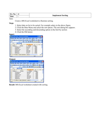
3. Ex. No. :1
Implement Sorting
Date :
Aim:
Steps
Input :
Create a MS-Excel worksheet to illustrate sorting.
1. Select data on list to be sorted. For example salary in the above figure.
2. Click the Data Menu and select the sort option. The sort dialog box appears.
3. Select the ascending and descending option in the Sort by section
4. Click the OK button
Output:
Result: MS-Excel worksheet created with sorting.

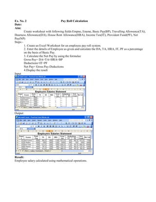
4. Ex. No. 2 Pay Roll Calculation
Date:
Aim:
Create worksheet with following fields Empno, Ename, Basic Pay(BP), Travelling Allowance(TA),
Dearness Allowance(DA), House Rent Allowance(HRA), Income Tax(IT), Provident Fund(PF), Net
Pay(NP)
Steps:-
Input
1. Create an Excel Worksheet for an employee pay roll system.
2. Enter the details of Employee as given and calculate the DA, TA, HRA, IT, PF as a percentage
on the basis of Basic Pay.
3. Calculate the Net Pay by using the formulae
Gross Pay= DA+TA+HRA+BP
Deductions=IT+PF
Net Pay= Gross Pay-Deductions
4.Display the result
Output:
Result:
Employee salary calculated using mathematical operations.

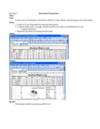
5. Ex. No.3 Mark Sheet Preparation
Date:
Aim:
Steps:
Input:
Create an Excel Worksheet with fields as Roll No, Name, Marks and percentage with chart display
1. Create an Excel Worksheet by inserting field names
2. Calculate total marks, Averages, Results and Divisions.(By using Mathematical and
Logical Functions)
3. Represent the Data by inserting the Pie Chart.
Output
Result:
The student marklist created using MS Excel

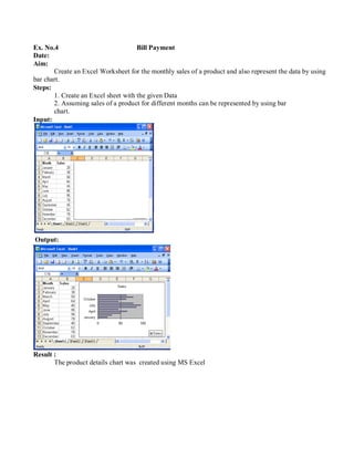
6. Ex. No.4 Bill Payment
Date:
Aim:
Create an Excel Worksheet for the monthly sales of a product and also represent the data by using
bar chart.
Steps:
Input:
1. Create an Excel sheet with the given Data
2. Assuming sales of a product for different months can be represented by using bar
chart.
Output:
Result :
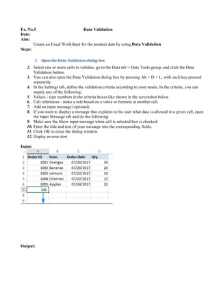
The product details chart was created using MS Excel

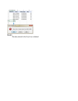
7. Ex. No.5 Data Validation
Date:
Aim:
Create an Excel Worksheet for the product data by using Data Validation
Steps:
1. Open the Data Validation dialog box
2. Select one or more cells to validate, go to the Data tab > Data Tools group, and click the Data
Validation button.
3. You can also open the Data Validation dialog box by pressing Alt > D > L, with each key pressed
separately.
4. In the Settings tab, define the validation criteria according to your needs. In the criteria, you can
supply any of the following:
5. Values - type numbers in the criteria boxes like shown in the screenshot below.
6. Cell references - make a rule based on a value or formula in another cell.
7. Add an input message (optional)
8. If you want to display a message that explains to the user what data is allowed in a given cell, open
the Input Message tab and do the following:
9. Make sure the Show input message when cell is selected box is checked.
10. Enter the title and text of your message into the corresponding fields.
11. Click OK to close the dialog window.
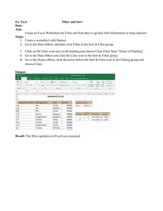
12. Display an error alert
Input:
Output:

8. Result :
The data entered in the Excel was validated

9. Ex. No.6 Filter and Sort
Date:
Aim:
Create an Excel Worksheet for Filter and Sort data to quickly find information in large datasets
Steps:
1. Create a worksheet with Dataset
2. Go to the Data ribbon, and then click Filter in the Sort & Filter group.
3. Click on the Filter icon next to the heading and choose Clear Filter from “Name of Heading”.
4. Go to the Data ribbon and click the Clear icon in the Sort & Filter group.
5. Go to the Home ribbon, click the arrow below the Sort & Filter icon in the Editing group and
choose Clear.
Output:
Result: The filter operation in Excel was executed

10. Ex. No. :7
Conditional Calculations(IF)
Date :
Aim:
Create an Excel Worksheet for IF statements to perform conditional calculations in your
spreadsheet.
Steps:
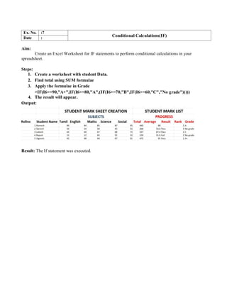
1. Create a worksheet with student Data.
2. Find total using SUM formulae
3. Apply the formulae in Grade
=IF(I6>=90,"A+",IF(I6>=80,"A",(IF(I6>=70,"B",IF(I6>=60,"C","No grade")))))
4. The result will appear.
Output:
Result: The If statement was executed.

11. Ex. No.8 Count If
Date:
Aim:
Steps:
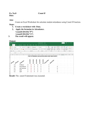
Create an Excel Worksheet for calculate student attendance using Count If Function.
1. Create a worksheet with Data.
2. Apply the formulae in Attendance.
=countif (D4:H4,”P”)
=countif (D4:H4,”A”)
3. The result will appear.
Output:
Result: The count If statement was executed.

12. Ex. No.9 Text Functions
Date:
Aim:
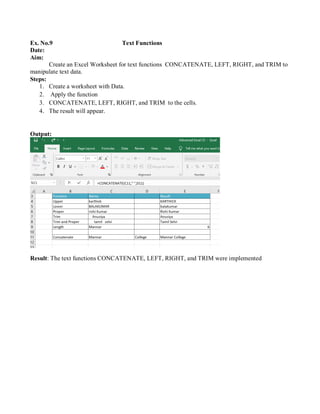
Create an Excel Worksheet for text functions CONCATENATE, LEFT, RIGHT, and TRIM to
manipulate text data.
Steps:
1. Create a worksheet with Data.
2. Apply the function
3. CONCATENATE, LEFT, RIGHT, and TRIM to the cells.
4. The result will appear.
Output:
Result: The text functions CONCATENATE, LEFT, RIGHT, and TRIM were implemented

13. Ex. No.10 VLOOKUP and HLOOKUP
Date:
Aim:
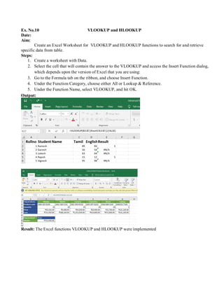
Create an Excel Worksheet for VLOOKUP and HLOOKUP functions to search for and retrieve
specific data from table.
Steps:
1. Create a worksheet with Data.
2. Select the cell that will contain the answer to the VLOOKUP and access the Insert Function dialog,
which depends upon the version of Excel that you are using:
3. Go to the Formula tab on the ribbon, and choose Insert Function.
4. Under the Function Category, choose either All or Lookup & Reference.
5. Under the Function Name, select VLOOKUP, and hit OK.
Output:
Result: The Excel functions VLOOKUP and HLOOKUP were implemented

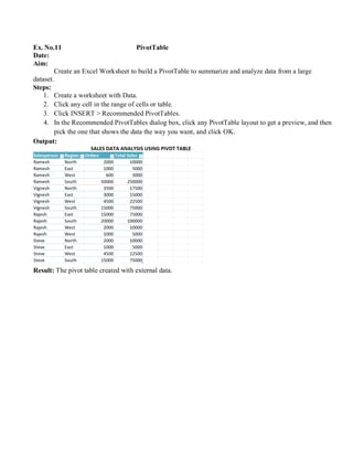
14. Ex. No.11 PivotTable
Date:
Aim:
Create an Excel Worksheet to build a PivotTable to summarize and analyze data from a large
dataset.
Steps:
1. Create a worksheet with Data.
2. Click any cell in the range of cells or table.
3. Click INSERT > Recommended PivotTables.
4. In the Recommended PivotTables dialog box, click any PivotTable layout to get a preview, and then
pick the one that shows the data the way you want, and click OK.
Output:
Result: The pivot table created with external data.

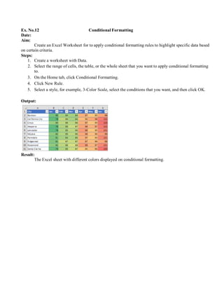
15. Ex. No.12 Conditional Formatting
Date:
Aim:
Create an Excel Worksheet for to apply conditional formatting rules to highlight specific data based
on certain criteria.
Steps:
1. Create a worksheet with Data.
2. Select the range of cells, the table, or the whole sheet that you want to apply conditional formatting
to.
3. On the Home tab, click Conditional Formatting.
4. Click New Rule.
5. Select a style, for example, 3-Color Scale, select the conditions that you want, and then click OK.
Output:
Result:
The Excel sheet with different colors displayed on conditional formatting.

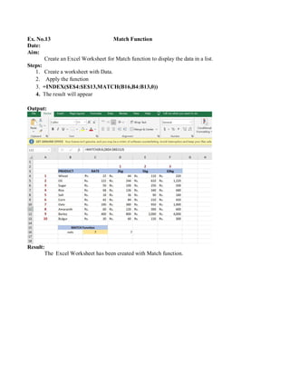
16. Ex. No.13 Match Function
Date:
Aim:
Create an Excel Worksheet for Match function to display the data in a list.
Steps:
1. Create a worksheet with Data.
2. Apply the function
3. =INDEX($E$4:$E$13,MATCH(B16,B4:B13,0))
4. The result will appear
Output:
Result:
The Excel Worksheet has been created with Match function.

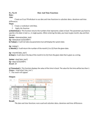
17. Ex. No.14 Date And Time Functions
Date:
Aim:
Create an Excel Worksheet to use date and time functions to calculate dates, durations and time
differences.
Steps:
1. Create a worksheet with Data.
2. Apply the function
a) DateValue( ):- This function returns the numbers that represents a date in Excel. The parameter you have to
specify is the date in text i.e., in single quotes. When entering the date, you have to give month, day and then
the year.
Syntax: =datevalue(date_text)
Eg: =datevalue(‘12/22/2007’)
b) Today( ):- It will not take any parameters but will display the system date.
Eg: =today( )
c) Month( ):- It will return the number of the month (1 to 12) from the given date.
Eg: =month(‘date_text’)
d) Day( ):- It will return the day of the month (1 to 31) from the given date that is given as a string.
Syntax: =day(‘date_text’)
Eg: =day(‘12/22/2007’)
Result: 22
e) Timevalue( ):- This function displays the value of the time in Excel. The value for the time will be less than 1.
Syntax: =timevalue(‘time_text’)
3 . The result will appear
Output:
Result:
The date and time functions were used and calculate dates, durations and time differences.

18. Ex. No. :15
Freeze The Cell And Text To Image Conversion
Date :
Aim:
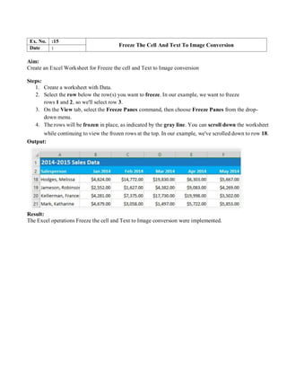
Create an Excel Worksheet for Freeze the cell and Text to Image conversion
Steps:
1. Create a worksheet with Data.
2. Select the row below the row(s) you want to freeze. In our example, we want to freeze
rows 1 and 2, so we'll select row 3.
3. On the View tab, select the Freeze Panes command, then choose Freeze Panes from the drop-
down menu.
4. The rows will be frozen in place, as indicated by the gray line. You can scroll down the worksheet
while continuing to view the frozen rows at the top. In our example, we've scrolled down to row 18.
Output:
Result:
The Excel operations Freeze the cell and Text to Image conversion were implemented.