Downloaded 289 times


![40
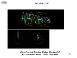
POLARIZATION
SOLO
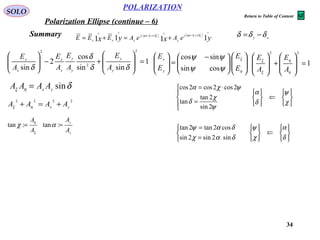
The Stokes Polarization Parameters (continue – 1)
We obtain
( ) ( ) ( ) ( ) ( )22222
sin2,4cos,,8,4 δδ yxyxyxyxxy
AAtzEAtzEtzEAAtzEA =+−
( ) ( ) ( ) ( )
( ) ( ) δδδωδδ
δωδω
δ
cos
2
22coscos
1
2
coscos
1
,,
0
0
lim
lim
yx
T
xyyx
T
yx
T
yxyx
T
zx
AA
dtzkt
T
AA
dtzktzktAA
T
tzEtzE
=
++−−−=
+−+−=
∫
∫
→∞
→∞
( ) ( ) ( )[ ]
2
2cos1
1
2
cos
1
,
2
0
2
0
222
limlim
x
T
x
T
x
T
xx
T
x
A
dtzkt
T
A
dtzktA
T
tzE =+−−=+−= ∫∫ →∞→∞
δωδω
( ) ( )
2
cos
1
,
2
0
222
lim
y
T
yy
T
y
A
dtzktA
T
tzE =+−= ∫→∞
δω
( ) ( )222222
sin22cos22 δδ yxyxyxyx
AAAAAAAA =+−
By adding and subtracting on the left side of this equation we obtain
( ) ( ) ( ) ( )22222222
sin2cos2 δδ yxyxyxyx
AAAAAAAA =−−−+
44
2 yx
AA +](https://image.slidesharecdn.com/polarization-141231132903-conversion-gate02/85/Polarization-40-320.jpg)


![46
POLARIZATION
SOLO
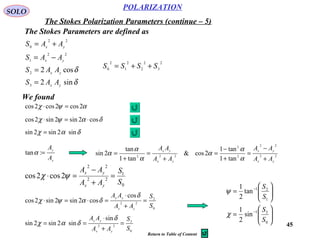
Consider a quasi-monochromatic wave of mean frequency ω propagating in z direction
composed of a Unpolarized component AUP with random phases δrx and δry and a
Polarized component Ax, δx , Ay, δy
( ) ( ) ( )tzkjj
yP
j
UP
j
xP
j
UPyx eeAeAeAeAEEE yxyx
yyrxxr ωδδδδ −−
∧∧∧∧
+++=+= 1111
Measuring the Stokes Parameters
Pass the beam through a waveplate that induces a wave retardation of φ and
a polarizer with a transmission axis at an angle β relative to x axis
( )
( ) ( )
( ) ( )tzkjj
yP
j
UP
j
xP
j
UP
eeAeAeAeAE yx
yyrxxr ωϕδδϕδδ −−
∧
−
∧
+
+++= 11
2/2/
'
( )
( ) ( )
( )[ ] ( )tzkjj
yP
j
UP
j
xP
j
UP
eeAeAeAeAE yyrxxr ωϕδδϕδδ
ββ −−−+
+++= sincos"
2/2/
The waveplate that induces a wave retardation of φ between the phases of x and y
components of the polarized light but will not affect the random phase of the unpolarized light.
The polarizer will transmit only the component along the transmission axis](https://image.slidesharecdn.com/polarization-141231132903-conversion-gate02/85/Polarization-46-320.jpg)
![47
POLARIZATION
SOLO
Measuring the Stokes Parameters (continue – 1)
( )
( ) ( )
( )[ ] ( )tzkjj
yP
j
UP
j
xP
j
UP
eeAeAeAeAE yyrxxr ωϕδδϕδδ
ββ −−−+
+++= sincos"
2/2/
( ) ( )
( ) ( )
( )[ ] ( )
( ) ( )
( )[ ] zz
yyrxxryyrxxr
j
yP
j
UP
j
xP
j
UP
j
yP
j
UP
j
xP
j
UP eAeAeAeAeAeAeAeAcnkEEcnkS 11 sincossincos"",
2/2/2/2/
∧
−−−+−−−+
∧
∗
+++⋅+++=⋅= ββββϕβ
ϕδδϕδδϕδδϕδδ
( )
( ) ( )
( )[ ] ( )
( ) ( )
( )[ ]
( ) ( )
( ) ( ) ( )
( ) ( )
( ) ( ) ( )
βββ
βββ
βββ
βββ
ββββ
ϕδδϕδδϕδδ
δϕδδϕδδδ
ϕδδϕδδδϕδ
δδδϕδδϕδ
ϕδδϕδδϕδδϕδδ
22
0
2/
0
2/
2
0
2/2
0
2/
0
2
0
2/22
0
2/
00
2/22
0
2/2
2/2/2/2/
sincossin
sin2/cossin
cossincos
cossincos2/
sincossincos
++
++
++
++
++
++
++
+=
+++⋅+++
−−−−−−−
−−−+−
−−+−−+
−−−−+
−−−+−−−+
yP
jj
yPUP
j
yPxP
jj
yPUP
jj
yPUPUP
jj
UPxP
jj
UP
j
xPyP
jj
xPUPxP
jj
xPUP
jj
UPyP
jj
UP
jj
xPUPUP
j
yP
j
UP
j
xP
j
UP
j
yP
j
UP
j
xP
j
UP
AeeAAeAAeeAA
eeAAAeeAAeeA
eAAeeAAAeeAA
eeAAeeAeeAAA
eAeAeAeAeAeAeAeA
yxpxyyxr
yyyrxyrrr
xyxyrxx
xryxryxrx
yyrxxryyrxxr
The time average Poynting vector is](https://image.slidesharecdn.com/polarization-141231132903-conversion-gate02/85/Polarization-47-320.jpg)
![48
POLARIZATION
SOLO
( ) ( )
( )[ ] zyP
jj
yPxPxPUP AeeAAAAcnkS 1
22222
sincossincos2/
∧
−−−
++++= ββββ ϕδϕδ
2
2sin
cossin
2
2cos1
sin
2
2cos1
cos
2
2
β
ββ
β
β
β
β
=
−
=
+
=
( ) ( ) ( ) ( )[ ]{ }
( ) ( ) ( ) ( )[ ]
( ) ( )[ ]
[ ]βϕβϕβ
βϕδβϕδβ
βϕβϕβ
βϕϕϕϕβ
δδδδ
δδ
2sinsin2sincos2cos
2
2sinsinsin22sincossin22cos
2
2sinsin2sincos2cos
2
2sinsincossincos2cos
2
********
22222
22222
22222
xyyxxyyxyyxxyyxx
yPxPyPxPyPxPyPxPUP
jj
yPxP
jj
yPxPyPxPyPxPUP
jj
yPxPyPxPyPxPUP
EEEEjEEEEEEEEEEEE
cnk
AAjAAAAAAA
cnk
eeAAjeeAAAAAAA
cnk
jejeAAAAAAA
cnk
S
−+++−++=
++−+++=
−−++−+++=
++−+−+++=
−−
−
Measuring the Stokes Parameters (continue – 2)
( )
( ) ( )
( )[ ] ( )
( ) ( )
( )[ ] zz
yyrxxryyrxxr
j
yP
j
UP
j
xP
j
UP
j
yP
j
UP
j
xP
j
UP eAeAeAeAeAeAeAeAcnkEEcnkS 11 sincossincos
2/2/2/2/
∧
−−−+−−−+
∧
∗
+++⋅+++=⋅= ββββ
ϕδδϕδδϕδδϕδδ
[ ]βϕβϕβ 2sinsin2sincos2cos
2
3210 SjSSS
cnk
S +++=
( )
( )
( )
( )xyyPxPxyyx
xyyPxPxyyx
yPxPyyxx
yPxPUPyyxx
AAEEEEjS
AAEEEES
AAEEEES
AAAEEEES
δδ
δδ
−=−=
−=+=
−=−=
++=+=
∗∗
∗∗
∗∗
∗∗
sin2
cos2
3
2
22
1
222
0](https://image.slidesharecdn.com/polarization-141231132903-conversion-gate02/85/Polarization-48-320.jpg)
![49
POLARIZATION
SOLO
Measuring the Stokes Parameters (continue – 3)
( ) [ ]βϕβϕβϕβ 2sinsin2sincos2cos
2
, 3210 SjSSS
cnk
S +++=
( )
( )
( )
( )xyyPxPxyyx
xyyPxPxyyx
yPxPyyxx
yPxPUPyyxx
AAEEEEjS
AAEEEES
AAEEEES
AAAEEEES
δδ
δδ
−=−=
−=+=
−=−=
++=+=
∗∗
∗∗
∗∗
∗∗
sin2
cos2
3
2
22
1
222
0
The Stokes Parameters are measured by first removing the waveplate φ = 0
( ) [ ]ββϕβ 2sin2cos
2
0, 210 SSS
cnk
S ++==
Now the polarizer is sequentially rotate to β = 0, π/4 and π/2
( ) [ ]10
2
0,0 SS
cnk
S +=== ϕβ
( ) [ ]20
2
0,4/ SS
cnk
S +=== ϕπβ
( ) [ ]10
2
0,2/ SS
cnk
S −=== ϕπβ
For the final measurement we
add the waveplate with φ = π/2
and polarizer at β = π/4
( ) [ ]30
2
2/,4/ SS
cnk
S −=== πϕπβ
( ) ( )[ ]0,2/0,0
2
0 ==+=== ϕπβϕβ SS
cnk
S
( ) ( )[ ]0,2/0,0
2
1 ==−=== ϕπβϕβ SS
cnk
S
( ) 02 0,4/2
2
SS
cnk
S −=== ϕπβ
( )2/,4/2
2
03
πϕπβ ==−= S
cnk
SS
](https://image.slidesharecdn.com/polarization-141231132903-conversion-gate02/85/Polarization-49-320.jpg)
![50
POLARIZATION
SOLO
Measuring the Stokes Parameters (continue – 4)
( ) [ ]βϕβϕβϕβ 2sinsin2sincos2cos
2
, 3210 SjSSS
cnk
S +++=
( )
( )
( )
( )xyyPxPxyyx
xyyPxPxyyx
yPxPyyxx
yPxPUPyyxx
AAEEEEjS
AAEEEES
AAEEEES
AAAEEEES
δδ
δδ
−=−=
−=+=
−=−=
++=+=
∗∗
∗∗
∗∗
∗∗
sin2
cos2
3
2
22
1
222
0
The Stokes Parameters can measure the degree of polarization of a beam.
We can see that a beam is unpolarized iff: 00 321
2
0
===>=+=
∗∗
SSSAEEEES UPyyxx
The Degree of Polarization is defined as: 10
0
2
3
2
2
2
1
222
22
≤≤
++
=
++
+
= P
S
SSS
AAA
AA
P
yPxPUP
yPxP
If the beam is completely polarized then AUP = 0: 0
2
3
2
2
2
1
2
0
>++= SSSS
Return to Table of Content](https://image.slidesharecdn.com/polarization-141231132903-conversion-gate02/85/Polarization-50-320.jpg)


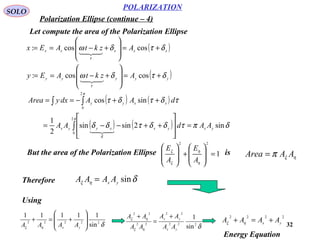
![68
POLARIZATION
SOLO
The Jones Polarization Parameters
R. Clark Jones, “A New Calculus for the Treatment of Optical Systems”,
J. Opt. Soc. Am., Vol.31, July 1941, pp.500-503
J. Opt. Soc. Am., Vol.32, Aug. 1942, pp.486-493
J. Opt. Soc. Am., Vol.37, Feb. 1947, pp.107-110
J. Opt. Soc. Am., Vol.37, Feb. 1947, pp.110-112
J. Opt. Soc. Am., Vol.38, Aug. 1948, pp.671-585 R. Clark Jones
1916-2004
Mueller matrices deal with the intensity of the beam. If the phase information
is important we must use Jones formalism.
Jones calculus was developed in the same time with the Mueller calculus by R.
Clark Jones who introduced Jones vectors and Jones matrices:
Jones vectors describe the
polarization of light:
Jones matrices describe
the optical component:
+
=
y
x
yx
E
E
EE
J
22
1
[ ]
=
2221
1211
jj
jj
J
Jones calculus deals only with polarized light.](https://image.slidesharecdn.com/polarization-141231132903-conversion-gate02/85/Polarization-68-320.jpg)


The document discusses polarization of light, including: 1) Natural or unpolarized light consists of randomly oriented electromagnetic waves from many emitters. Monochromatic planar waves can be linearly, circularly, or elliptically polarized depending on their wave properties. 2) Several methods can achieve polarization, including dichroism via materials that selectively absorb certain orientations, scattering, reflection using Brewster's angle, and birefringence in crystals. 3) Key polarization components are described like polarizers using dichroic materials, wire grids, reflection, and birefringent prisms made of crystals like calcite or quartz. Polarization ellipses represent the tip trajectory of the oscillating electric field


