Downloaded 182 times


![31
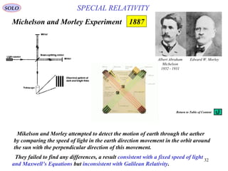
SOLO
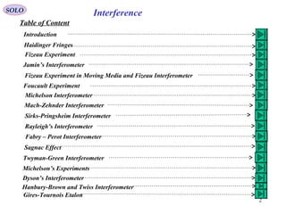
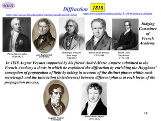
Michelson Interferometer – Broad Source
Interference 1882 Nobel Prize 1907
José Antonio Diaz Navas
http://www.ugr.es/~jadiaz/
[ ]
+
+
+∆
−++= π
λ
π
υπ
f
yx
d
Logc
yx
f
d
IIIII
22
22
2121 2cos
2
cos
2
1
cos
exp2
I – intensity of the interference fringes
I1, I2 – intensity of the intensities of the two beams
λ, c – wavelength, speed of light
d – path length difference between the two
interferometers arms
x,y – coordinates of the focal plane of a lens of
focal length f
The intensity of the interference fringes for a Michelson interferometer having a source emitting
with a Gaussian profile having a bandwidth of Δν is given by](https://image.slidesharecdn.com/interferometershistory-150105104817-conversion-gate01/85/Interferometers-history-31-320.jpg)


![43
InterferenceSOLO
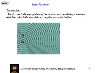
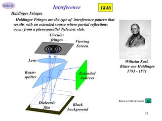
Interference of Two Monochromatic Waves
Given two waves ( ω = constant ):
( ) ( ) ( )[ ]{ } ( ){ }tUtiAtAtu 111111 ReexpRecos =+=+= φωφω
where the corresponding phasors, are defined as:
( ) ( )[ ]111 exp: φω += tiAtU
The two waves interfere to give:
( ) ( ) ( ) ( ) ( )
( ) ( ){ } ( )φω
φωφω
+=+=
+++=+=
tAtUtU
tAtAtututu
cosRe
coscos
21
221121
( ) ( ) ( )[ ]{ } ( ){ }tUtiAtAtu 222222 ReexpRecos =+=+= φωφω
( ) ( )[ ]222 exp: φω += tiAtU
1
U
2
U
21 UUU +=
1φ2φ φ
( )1221
2
2
2
1
212211
cos2
2
φφ −⋅⋅++=
⋅⋅+⋅+⋅==
∗∗∗
AAAA
UUUUUUUA
2
U
( )
+
+
=
−++=
−
2211
22111
2121
2
2
2
1
coscos
sinsin
tan
cos2
φφ
φφ
φ
φφ
AA
AA
AAAAA
The Phasor summation
is identical to
Vector summation](https://image.slidesharecdn.com/interferometershistory-150105104817-conversion-gate01/85/Interferometers-history-43-320.jpg)
![44
InterferenceSOLO
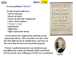
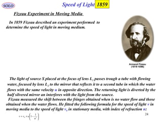
Interference of Monochromatic Waves
Given two electromagnetic monochromatic ( ω = constant ) waves:
( ) ( ) ( ) ( ) ( )[ ]{ } ( ){ }trErktirErktrEtrE ,ReexpRecos, 1111110111110111
=+⋅−=+⋅−= φωφω
( ) ( ) ( ) ( ) ( )[ ]{ } ( ){ }trErktirErktrEtrE ,ReexpRecos, 2222220222220222
=+⋅−=+⋅−= φωφω
where the corresponding phasors, are defined as:
( ) ( ) ( )[ ]11110111 exp:, φω +⋅−= rktirEtrE
( ) ( ) ( )[ ]22220222
exp:, φω +⋅−= rktirEtrE
1
S
2
S
P
1r
2
r
2211 1
2
:&1
2
: rkrk
λ
π
λ
π
==
At the point P the two waves interfere to give:
( ) ( ) ( ) ( ) ( ) ( ) ( )
( ) ( ){ }trEtrE
rktrErktrEtrEtrEtrE
,,Re
coscos,,,
2211
2222021111012211
+=
+⋅−++⋅−=+= φωφω
The Irradiance at the point P is given by:
( ) ( ) ( ) ( )trHtrHtrEtrEI ,,,,
∗∗
⋅=⋅= µε](https://image.slidesharecdn.com/interferometershistory-150105104817-conversion-gate01/85/Interferometers-history-44-320.jpg)
![45
InterferenceSOLO
Interference of Monochromatic Waves
1S
2S
P
1
r
2
r
The Irradiance at the point P is given by:
( ) ( ) ( ) ( )[ ] ( ) ( )[ ]
( ) ( ) ( ) ( ) ( ) ( ) ( ) ( )trEtrEtrEtrEtrEtrEtrEtrE
trEtrEtrEtrEtrEtrEI
,,,,,,,,
,,,,,,
1122221122221111
22112211
∗∗∗∗
∗∗∗
⋅+⋅+⋅+⋅=
+⋅+=⋅=
εεεε
εε
( ) ( ) ( ) ( )10110111111
,, rErEtrEtrEI
⋅=⋅=
∗
εε
( ) ( ) ( ) ( )20220222222 ,, rErEtrEtrEI
⋅=⋅=
∗
εε
( ) ( ) ( ) ( )
( ) ( )[ ] ( ) ( )[ ]
( ) ( )[ ] ( ) ( )[ ]
( ) ( ) ( )[ ] ( )[ ]{ }
( ) ( ) ( ) ( )21112221211122202101
211122211122202101
111101222202
222202111101
1122221112
cos2cos2
expexp
expexp
expexp
,,,,
φφφφε
φφφφε
φωφωε
φωφωε
εε
−+⋅−⋅=−+⋅−⋅⋅=
−+⋅−⋅−+−+⋅−⋅⋅=
+⋅−−⋅+⋅−+
+⋅−−⋅+⋅−=
⋅+⋅=
∗∗
rkrkIIrkrkrErE
rkrkirkrkirErE
rktirErktirE
rktirErktirE
trEtrEtrEtrEI
( )21112221211221
cos2 φφ −+⋅−⋅++=++= rkrkIIIIIIII
](https://image.slidesharecdn.com/interferometershistory-150105104817-conversion-gate01/85/Interferometers-history-45-320.jpg)


![50
SOLO
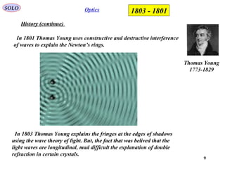
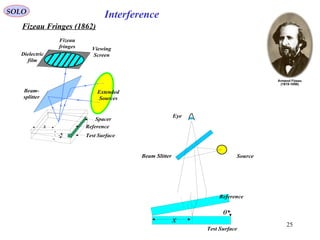
Young’s Experiment (continue – 1)
s
a
yrr
sa<<
≈− 12
The bright fringes are obtained when:
,2,1,012
±±==− mmrr λ
,2,1,0 ±±== mm
s
a
y λ
The distance between two consecutive
bright fringes is:
( ) λλλ
a
s
a
s
m
a
s
myyy mm =−+≈−=∆ + 11
The dark fringes are obtained when:
,2,1,0
2
12
±±=+=− mmrr
λ
λ
( ) ,2,1,0
2
12 ±±=+= mm
s
a
y
λ
λ - wavelength
The Intensity at point P is:
( ) ( )[ ]{ }
=−+=−+⋅−⋅++=
=
−=−
==
=
s
ya
IrrkIrkrkIIIII
k
syarr
III
λ
π
φφ
λπ
φφ
2
0
/2
/
1202111222121 cos4cos12cos2
12
021
21
1r
2r
s
a
y
2S
1S
P
OS 'O
aΣ oΣ
http://homepage.univie.ac.at/Franz.Embacher/KinderUni2005/waves.gif
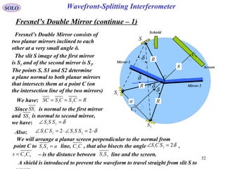
Wavefront-Splitting Interferometer
Classes of InterferometersReturn to Table of Content](https://image.slidesharecdn.com/interferometershistory-150105104817-conversion-gate01/85/Interferometers-history-50-320.jpg)


![55
SOLO
Fresnel’s Double Prism
The Fresnel’s Double Prism or Bi-prism
consists of two thin prisms joined at their
bases. A singlr cylindrical wave emerge from
a slit. The top part of the wave-front is
Refracted downward, and the lower segment
is refracted upward. In the region of
superposition interference occurs.
Screen
Bi-prism
Slit
y
z
δ
s
a
2S
1
S
O
S 'O
aΣ
o
Σ
1<<α
iθ
d
iθ - incident angle
δ - dispersion angle
α - prism angle
From the Figure we can see that two
virtual sources S1 and S2 exists. Let a
be the distance between them.
From the Figure
( ) δδθθ
θ
δ
ddd
a i
ii
1
1
sintan
2
<<
<<
≈−−=
where
θi – ray incident angle
δ – ray dispersion (deviation) angle
d – distance slit to bi-prism vertex
α – prism angle
( )[ ]
[ ] ( )ααθαθ
αθαθαθδ
α
θ
α
θ
1sin
sincossinsinsin
1
1
1
1
1
2/1221
−≈−−+≈
−−−+=
<<
<<
−
<<
<<
−
nn
n
n
ii
iii
ii
See δ development
Wavefront-Splitting Interferometer](https://image.slidesharecdn.com/interferometershistory-150105104817-conversion-gate01/85/Interferometers-history-55-320.jpg)
![56
SOLO
Dispersive Prisms
( ) ( )2211 itti
θθθθδ −+−=
21 it
θθα +=
αθθδ −+= 21 ti
202
sinsin ti
nn θθ =Snell’s Law
10
≈n
( ) ( )[ ]1
1
2
1
2
sinsinsinsin tit
nn θαθθ −== −−
( )[ ] ( )[ ]11
21
11
1
2 sincossin1sinsinsincoscossinsin ttttt nn θαθαθαθαθ −−=−= −−
Snell’s Law 110
sinsin ti
nn θθ =
11
sin
1
sin it
n
θθ =
10
≈n
( )[ ]1
2/1
1
221
2 sincossinsinsin iit n θαθαθ −−= −
( )[ ] αθαθαθδ −−−+= −
1
2/1
1
221
1
sincossinsinsin iii
n
The ray deviation angle is
Optics - Prisms](https://image.slidesharecdn.com/interferometershistory-150105104817-conversion-gate01/85/Interferometers-history-56-320.jpg)
![57
SOLO
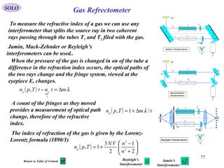
Fresnel’s Double Prism (continue – 1)
From the Figure we found that the distance a
between virtual sources S1 and S2 is:
( ) δδθθ
θ
δ
ddd
a i
ii
1
1
sintan
2
<<
<<
≈−−=
( )[ ]
[ ] ( )ααθαθ
αθαθαθδ
α
θ
α
θ
1sin
sincossinsinsin
1
1
1
1
1
2/1221
−≈−−+≈
−−−+=
<<
<<
−
<<
<<
−
nn
n
n
ii
iii
ii
See δ development
( )α12 −≈ nda
s
a
y
2S
1
S P
OS 'O
aΣ o
Σ
1<<α
α - prism angle
1r
2r
Screen
Bi-prism
Slit
y
z
Consider two rays starting from the slit S that
pass the bi-prism and interfere on the screen
at P. We can assume that they are strait lines
starting at the virtual source S1 and S2, and
having optical paths r1 and r2, respectively.
2
2
2
22
2
2
2
11
22
zy
a
sPSrzy
a
sPSr +
++==+
−+==
Wavefront-Splitting Interferometer
δ
s
a
2S
1
S
O
S 'O
a
Σ
o
Σ
1<<α
iθ
d
iθ - incident angle
δ - dispersion angle
α - prism angle](https://image.slidesharecdn.com/interferometershistory-150105104817-conversion-gate01/85/Interferometers-history-57-320.jpg)


![65
SOLO
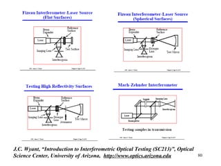
Optical Reflected Path Length Difference: Parallel Interfaces (continue – 2)
Two-Beam Interference: Parallel Interfaces
'D
1
θ
1
θ
1
θ 2θ
2
θ
d
C
B
D
1n
2
n
1
n
Point
source
Image
1
2
Dielectric
slab
( ) ( )
−=
0
1
12
'2
exp'
λ
π
ωθ
BDn
tirADE
( ) ( ) ( )
+
+
−= π
λ
π
ωθ
0
2
11
2
exp
CDBCn
tirADE
2cos/ θdCDBC ==
From the Figure we obtain:
12 sintan2' θθdBD =
The phase difference at interference is:
( )[ ] π
λ
π
φφ +−+−=− BDnCDBCn 12
0
21
2
2
2
2
2
sinsin
1
2
2
1121
cos
sin
sin
cos
sin
sintan
2211
θ
θ
θ
θ
θ
θθ
θθ
nnn
nn =
==
( ) πθ
λ
π
πθ
θλ
π
πθθ
θλ
π
φφ +−=+
−−=+
−−=− 2
0
2
2
2
2
2
0
121
2
2
0
21 cos
4
sin1
cos
22
sintan
cos
2
2 ndnd
n
n
d
Amplitude Split Interferometers](https://image.slidesharecdn.com/interferometershistory-150105104817-conversion-gate01/85/Interferometers-history-65-320.jpg)

![67
SOLO
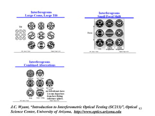
Optical Transmitted Path Length Difference: Parallel Interfaces
Two-Beam Interference: Parallel Interfaces
Amplitude Split Interferometers
( ) ( ) ( )
+
−=
0
12
12
'2
exp'
λ
π
ωθ
BDnABn
tirADE
( ) ( ) ( )
+
++
−= π
λ
π
ωθ
0
2
11
2
exp
CDBCABn
tirADE
2cos/ θdCDBCAB ===
From the Figure we obtain:
12 sintan2' θθdBD =
The phase difference at interference is:
( )[ ] π
λ
π
φφ +−+−=− '
2
12
0
21 BDnCDBCn
2
2
2
2
sinsin
1
2
2
1121
cos
sin
sin
cos
sin
sintan
2211
θ
θ
θ
θ
θ
θθ
θθ
nnn
nn =
==
( ) πθ
λ
π
πθ
θλ
π
πθθ
θλ
π
φφ +−=+
−−=+
−−=− 2
0
2
2
2
2
2
0
121
2
2
0
21
cos
4
sin1
cos
22
sintan
cos
2
2 ndnd
n
n
d
( ) ( ) ( ) ( )01
0
2
10 exp
2
exp δωθ
λ
π
ωθ −=
−= tirA
ABn
tirABE
2
0
2
20
2
0
cos
4
:
cos
2
:
θ
λ
π
δ
θλ
π
δ
nd
nd
=
=
Return to Table of Content](https://image.slidesharecdn.com/interferometershistory-150105104817-conversion-gate01/85/Interferometers-history-67-320.jpg)


![70
InterferenceSOLO
Interference of Many Monochromatic Waves
Given two waves ( ω = constant ):
( ) ( ) ( )[ ]{ } ( ){ }tUtiAtAtu 111111 ReexpRecos =+=+= φωφω
The N waves interfere to give:
( ) ( ) ( ) ( )
( ) ( ) ( ){ } ( )φω +=+++=
+++=
tAtUtUtU
tutututu
N
N
cosRe 21
21
( ) ( ) ( )[ ]{ } ( ){ }tUtiAtAtu 222222 ReexpRecos =+=+= φωφω
1U
N
UUUU +++= 21
1φ
2φ
φ
2
U
N
U
Nφ
The Phasor summation is identical to Vector summation
( ) ( ) ( )[ ]{ } ( ){ }tUtiAtAtu NNNNNN ReexpRecos =+=+= φωφω](https://image.slidesharecdn.com/interferometershistory-150105104817-conversion-gate01/85/Interferometers-history-70-320.jpg)

![72
InterferenceSOLO
Multiple Beam Interference from a Parallel Film
( )
( )
( )[ ]
δω
δω
δω
ω
1
0
32
2
0
3
3
02
01
''
''
''
−−−
−
−
=
=
=
=
NtiN
rN
ti
r
ti
r
ti
r
eEtrtE
eEtrtE
eEtrtE
eErE
We have:
We have a point source and a dielectric slab that performs a multiple reflection and
transmission.
( )
( )
( ) ( )[ ]
δωδ
δωδ
δωδ
ωδ
1
0
12
2
0
4
3
0
2
2
01
0
0
0
0
''
''
''
'
−−−−
−−
−−
−
=
=
=
=
NtiiN
rN
tii
t
tii
t
tii
t
eeEtrtE
eeEtrtE
eeEtrtE
eeEttE 2
0
2
20
2
0
cos
4
:
cos
2
:
θ
λ
π
δ
θλ
π
δ
nd
nd
=
=](https://image.slidesharecdn.com/interferometershistory-150105104817-conversion-gate01/85/Interferometers-history-72-320.jpg)
![73
InterferenceSOLO
Multiple Beam Interference from a Parallel Film
Using lens the multi-rays interfere at lens focus.
( )
[ ] tiNiNii
rNrrr
eEetrtetrtetrtr
EEEE
ωδδδ
0
13223
21
''''''
+++++=
++++=
−−−−−
( )
ti
i
NiN
i
eE
er
er
etrtr ω
δ
δ
δ
02
132
'1
'1
''
−
−
+= −
−−−
−
∞→
<
Nand
rIf 1' ti
i
i
r eE
er
etrt
rE ω
δ
δ
02
'1
''
−
+= −
−
In the case of zero absorption, no energy being
taken out of the waves, using Stokes relations
2
1'&' rttrr −=−=
( ) ti
i
i
r eE
er
er
E ω
δ
δ
02
1
1
−
−
= −
−
∞→
<
Nand
rIf 1](https://image.slidesharecdn.com/interferometershistory-150105104817-conversion-gate01/85/Interferometers-history-73-320.jpg)
![74
InterferenceSOLO
Multiple Beam Interference from a Parallel Film
Using lens the multi-rays interfere at lens focus.
( ) ( )
[ ] ( )0
0
112242
21
''''1 δωδδδ −−−−−−
+++++=
++++=
tiNiNii
tNttt
eEttererer
EEEE
( )0
02
2
'
'1
'1 δω
δ
δ
−
−
−
−
−
= ti
i
NiN
eEtt
er
er
∞→
<
Nand
rIf 1' ( )0
02
'1
' δω
δ
−
−
−
= ti
it eE
er
tt
E
In the case of zero absorption, no energy being
taken out of the waves, using Stokes relations
2
1'&' rttrr −=−=
( )0
02
2
1
1 δω
δ
−
−
−
−
= ti
it eE
er
r
E
2
0
2
20
2
0
cos
4
:
cos
2
:
θ
λ
π
δ
θλ
π
δ
nd
nd
=
=](https://image.slidesharecdn.com/interferometershistory-150105104817-conversion-gate01/85/Interferometers-history-74-320.jpg)
![75
InterferenceSOLO
Multiple Beam Interference from a Parallel Film
∞→
<
Nand
rIf 1
( ) ti
i
i
r eE
er
er
E ω
δ
δ
02
1
1
−
−
= −
−
( )0
02
2
1
1 δω
δ
−
−
−
−
= ti
it eE
er
r
E
Let compute the Reflected and Transmitted
Irradiances:
( ) ( ) ( )
( ) 024
2
*
0022
*
cos21
cos12
1
1
1
1
I
rr
r
EE
er
er
er
er
EEI i
i
i
i
rrr
δ
δ
δ
δ
δ
δ
−+
−
=
−
−
−
−
=∝ −
−
( )
( ) 024
22
*
002
2
2
2
*
cos21
1
1
1
1
1
I
rr
r
EE
er
r
er
r
EEI iittt
δδδ
−+
−
=
−
−
−
−
=∝ −
Using lens the multi-rays interfere at lens focus we found
that in the case of zero absorption, no energy
being taken out of the waves, using Stokes
relations
2
1'&' rttrr −=−=
0III tr =+
( ) ( )[ ] ( )
( )[ ] ( )
0222
2222/sin21cos
2/sin1/21
2/sin1/2
2
I
rr
rr
Ir
δ
δδδ
−+
−
=
−=
( )
( )[ ] ( )
0222
2/sin21cos
2/sin1/21
1
2
I
rr
It
δ
δδ
−+
=
−=
We see that](https://image.slidesharecdn.com/interferometershistory-150105104817-conversion-gate01/85/Interferometers-history-75-320.jpg)


The document provides a comprehensive overview of the history and development of interferometry, diffraction, and optics, highlighting key experiments and scientists from the 17th to 19th centuries. It details significant contributions from figures like Fizeau, Young, Hooke, Newton, and Fresnel, while elucidating concepts such as light waves, interference, refraction, and diffraction patterns. The text also discusses various experimental setups and their implications for understanding the behavior of light.


