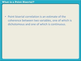
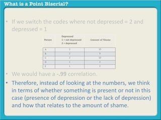
Point biserial correlation measures the relationship between one dichotomous variable (having two possible values) and one continuous variable (having a range of possible values). It ranges from -1 to 1. An example is measuring the correlation between depression status (depressed or not depressed) and self-reported shame levels (on a scale of 1 to 10). The direction of the correlation depends on how the variables are coded, with higher values representing more of the attribute.

1. Point Biserial Correlation
Welcome to the Point Biserial
Correlation Conceptual Explanation

2. • Point biserial correlation is an estimate of the
coherence between two variables, one of which is
dichotomous and one of which is continuous.

3. • Point biserial correlation is an estimate of the
coherence between two variables, one of which is
dichotomous and one of which is continuous.
Coherence means how much the
two variables covary.

4. • Let’s look at an example of two variables cohering

5. • The data set below represents the average decibel
levels at which different age groups listen to music.

6. • The data set below represents the average decibel
levels at which different age groups listen to music.
Age Group Decibels
80s 30
70s 35
60s 37
50s 39
40s 45
30s 50
20s 75
Teens 95

7. • The data set below represents the average decibel
levels at which different age groups listen to music.
Age Group Decibels
80s 30
70s 35
60s 37
50s 39
40s 45
30s 50
20s 75
Teens 95
The reason these two variables (age group and
decibel level) cohere is because as one increases
the other either increases or decreases
commensurately.

8. • The data set below represents the average decibel
levels at which different age groups listen to music.
In this case
Age Group Decibels
80s 30
70s 35
60s 37
50s 39
40s 45
30s 50
20s 75
Teens 95

9. • The data set below represents the average decibel
levels at which different age groups listen to music.
In this case as age goes up
Age Group Decibels
80s 30
70s 35
60s 37
50s 39
40s 45
30s 50
20s 75
Teens 95

10. • The data set below represents the average decibel
levels at which different age groups listen to music.
In this case as age goes up
Age Group Decibels
80s 30
70s 35
60s 37
50s 39
40s 45
30s 50
20s 75
Teens 95

11. • The data set below represents the average decibel
levels at which different age groups listen to music.
In this case as age goes up, decibels go down
Age Group Decibels
80s 30
70s 35
60s 37
50s 39
40s 45
30s 50
20s 75
Teens 95

12. • The data set below represents the average decibel
levels at which different age groups listen to music.
In this case as age goes up, decibels go down
Age Group Decibels
80s 30
70s 35
60s 37
50s 39
40s 45
30s 50
20s 75
Teens 95

13. • The data set below represents the average decibel
levels at which different age groups listen to music.
In this case as age goes up, decibels go down
Age Group Decibels
80s 30
70s 35
60s 37
50s 39
40s 45
30s 50
20s 75
Teens 95
• This is called a negative relationship.

14. • It is called a negative correlation or coherence,
because when one variable increases, the other
decreases (or vice-a-versa)

15. • A positive correlation would occur when as one
variable increases, the other increases or when one
decreases the other decreases.

16. • A positive correlation would occur when as one
variable increases, the other increases or when one
decreases the other decreases.

17. • A positive correlation would occur when as one
variable increases, the other increases or when one
decreases the other decreases.
• Example

18. • A positive correlation would occur when as one
variable increases, the other increases or when one
decreases the other decreases.
• Example
• As the temperature rises the average daily purchase
of popsicles increases.

19. • A positive correlation would occur when as one
variable increases, the other increases or when one
decreases the other decreases.
• Example
• As the temperature rises the average daily purchase
of popsicles increases.
Average Daily Temp
Average Daily
Popsicle Purchases
Per Person
100 2.30
95 1.20
90 1.00
85 .80
80 .70
75 .10
70 .03
65 .01

20. • A positive correlation would occur when as one
variable increases, the other increases or when one
decreases the other decreases.
• Example
• As the temperature rises the average daily purchase
of popsicles increases.
Average Daily Temp
Average Daily
Popsicle Purchases
Per Person
100 2.30
95 1.20
90 1.00
85 .80
80 .70
75 .10
70 .03
65 .01

21. • A positive correlation would occur when as one
variable increases, the other increases or when one
decreases the other decreases.
• Example
• As the temperature rises the average daily purchase
of popsicles increases.
Average Daily Temp
Average Daily
Popsicle Purchases
Per Person
100 2.30
95 1.20
90 1.00
85 .80
80 .70
75 .10
70 .03
65 .01
• These variables are positively correlated because as
one variable (Daily Temp) increases another variable
(average daily popsicle purchase) increases.

22. • It can be stated another way:

23. • It can be stated another way:
• As the average daily temperature decreases the
average daily popsicle purchases decrease as well.

24. • It can be stated another way:
• As the average daily temperature decreases the
average daily popsicle purchases decrease as well.
Average Daily Temp
Average Daily
Popsicle Purchases
Per Person
100 2.30
95 1.20
90 1.00
85 .80
80 .70
75 .10
70 .03
65 .01

25. • It can be stated another way:
• As the average daily temperature decreases the
average daily popsicle purchases decrease as well.
Average Daily Temp
Average Daily
Popsicle Purchases
Per Person
100 2.30
95 1.20
90 1.00
85 .80
80 .70
75 .10
70 .03
65 .01

26. • It can be stated another way:
• As the average daily temperature decreases the
average daily popsicle purchases decrease as well.
Average Daily Temp
Average Daily
Popsicle Purchases
Per Person
100 2.30
95 1.20
90 1.00
85 .80
80 .70
75 .10
70 .03
65 .01
• These variables are also positively correlated
because as one variable (Daily Temp) decreases
another variable (average daily popsicle purchase)
decreases.

27. • Let’s return to our Point Biserial Correlation
definition:

28. • Let’s return to our Point Biserial Correlation
definition:
• “Point biserial correlation is an estimate of the
coherence between two variables, one of which is
dichotomous and one of which is continuous.”

29. • Let’s return to our Point Biserial Correlation
definition:
• “Point biserial correlation is an estimate of the
coherence between two variables, one of which is
dichotomous and one of which is continuous.”
We discussed coherence

30. • Let’s return to our Point Biserial Correlation
definition:
• “Point biserial correlation is an estimate of the
coherence between two variables, one of which is
dichotomous and one of which is continuous.”
But, what is a dichotomous
variable?

31. • A dichotomous variable is a variable that can only be
one thing or another.

32. • A dichotomous variable is a variable that can only be
one thing or another.
• Here are some examples:

33. • A dichotomous variable is a variable that can only be
one thing or another.
• Here are some examples:
– When you can only answer “Yes” or “No”

34. • A dichotomous variable is a variable that can only be
one thing or another.
• Here are some examples:
– When you can only answer “Yes” or “No”
– When your statement can only be categorized as “Fact” or “Opinion”

35. • A dichotomous variable is a variable that can only be
one thing or another.
• Here are some examples:
– When you can only answer “Yes” or “No”
– When your statement can only be categorized as “Fact” or “Opinion”
– When you are either are something or you are not “Catholic” or “Not
Catholic”

36. • The dichotomous variable may be naturally occurring
as in gender

37. • The dichotomous variable may be naturally occurring
as in gender

38. • The dichotomous variable may be naturally occurring
as in gender
• or may be arbitrarily dichotomized as in
depressed/not depressed.

39. • The dichotomous variable may be naturally occurring
as in gender
• or may be arbitrarily dichotomized as in
depressed/not depressed.

40. • The range of a point biserial correlation in from -1 to +1.

41. • The range of a point biserial correlation in from -1 to +1.
-1 0 +1

42. • Let’s return again to our Point Biserial Correlation
definition:

43. • Let’s return again to our Point Biserial Correlation
definition:
• “Point biserial correlation is an estimate of the
coherence between two variables, one of which is
dichotomous and one of which is continuous.”

44. • Let’s return again to our Point Biserial Correlation
definition:
• “Point biserial correlation is an estimate of the
coherence between two variables, one of which is
dichotomous and one of which is continuous.”

45. • Let’s return again to our Point Biserial Correlation
definition:
• “Point biserial correlation is an estimate of the
coherence between two variables, one of which is
dichotomous and one of which is continuous.”
So, we now know what a
dichotomous variable is
(either / or)

46. • Let’s return again to our Point Biserial Correlation
definition:
• “Point biserial correlation is an estimate of the
coherence between two variables, one of which is
dichotomous and one of which is continuous.”

47. • Let’s return again to our Point Biserial Correlation
definition:
• “Point biserial correlation is an estimate of the
coherence between two variables, one of which is
dichotomous and one of which is continuous.”
What is a continuous
variable?

48. • Definition of Continuous Variable:

49. • Definition of Continuous Variable:
• If a variable can take on any value between its minimum
value and its maximum value, it is called a continuous
variable.

50. • Definition of Continuous Variable:
• If a variable can take on any value between its minimum
value and its maximum value, it is called a continuous
variable.
• Here is an example:

51. • Definition of Continuous Variable:
• If a variable can take on any value between its minimum
value and its maximum value, it is called a continuous
variable.
• Here is an example:
Suppose the fire department mandates that all fire fighters must weigh
between 150 and 250 pounds. The weight of a fire fighter would be an example
of a continuous variable; since a fire fighter's weight could take on any value
between 150 and 250 pounds.

52. • Definition of Continuous Variable:
• If a variable can take on any value between its minimum
value and its maximum value, it is called a continuous
variable.
• Here is an example:
Suppose the fire department mandates that all fire fighters must weigh
between 150 and 250 pounds. The weight of a fire fighter would be an example
of a continuous variable; since a fire fighter's weight could take on any value
between 150 and 250 pounds.

53. • The direction of the correlation depends on how the
variables are coded.

54. • The direction of the correlation depends on how the
variables are coded.
• Let’s say we are comparing the shame scores
(continuous variable from 1-10) and whether someone
is depressed or not (dichotomous variable – not
depressed = 1 and depressed = 2). .

55. • If the dichotomous variable is coded with the higher
value representing the presence of an attribute
(depressed)

56. • If the dichotomous variable is coded with the higher
value representing the presence of an attribute
(depressed)
Person
Depressed
1 = not depressed
2 = depressed
A
B
C
D
E

57. • If the dichotomous variable is coded with the higher
value representing the presence of an attribute
(depressed)
Person
Depressed
1 = not depressed
2 = depressed
A Depressed
B Depressed
C Depressed
D Not Depressed
E Not Depressed

58. • If the dichotomous variable is coded with the higher
value representing the presence of an attribute
(depressed)
Person
Depressed
1 = not depressed
2 = depressed
A 2
B 2
C 2
D 1
E 1

59. • . . . and the continuous variable is coded with higher
values representing the increasing presence of an
attribute (shame),

60. • . . . and the continuous variable is coded with higher
values representing the increasing presence of an
attribute (shame),
Person
Depressed
1 = not depressed
2 = depressed
Amount of Shame
A 2 10
B 2 9
C 2 10
D 1 2
E 1 2

61. • . . . and the continuous variable is coded with higher
values representing the increasing presence of an
attribute (shame),
Person
Depressed
1 = not depressed
2 = depressed
Amount of Shame
A 2 10
B 2 9
C 2 10
D 1 2
E 1 2
• then positive values of the point-biserial would indicate
higher shame associated with depressed status. In this
case we would compute a phi-coefficient of +.99

62. • . . . and the continuous variable is coded with higher
values representing the increasing presence of an
attribute (shame),
Person
Depressed
1 = not depressed
2 = depressed
Amount of Shame
A 2 10
B 2 9
C 2 10
D 1 2
E 1 2
• then positive values of the point-biserial would indicate
higher shame associated with depressed status. In this
case we would compute a Point Biserial of +.99

63. • If we switch the codes where not depressed = 2 and
depressed = 1

64. • If we switch the codes where not depressed = 2 and
depressed = 1
Person
Depressed
1 = not depressed
2 = depressed
Amount of Shame
A 1 10
B 1 9
C 1 10
D 2 2
E 2 2

65. • If we switch the codes where not depressed = 2 and
depressed = 1
Person
Depressed
1 = not depressed
2 = depressed
Amount of Shame
A 1 10
B 1 9
C 1 10
D 2 2
E 2 2
• We would have a -.99 correlation.

66. • If we switch the codes where not depressed = 2 and
depressed = 1
Person
Depressed
1 = not depressed
2 = depressed
Amount of Shame
A 1 10
B 1 9
C 1 10
D 2 2
E 2 2
• We would have a -.99 correlation.

67. • If we switch the codes where not depressed = 2 and
depressed = 1
Person
Depressed
1 = not depressed
2 = depressed
Amount of Shame
A 2 10
B 2 9
C 2 10
D 1 2
E 1 2
• We would have a -.99 correlation.
• Therefore, instead of looking at the numbers, we think
in terms of whether something is present or not in this
case (presence of depression or the lack of depression)
and how that relates to the amount of shame.

68. • The strength of the association can be tested against
chance just as the Pearson Product Moment Correlation
Coefficient.