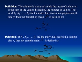
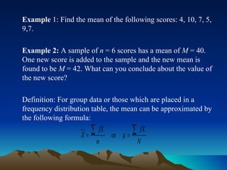
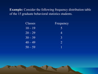
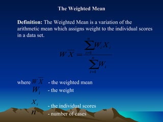
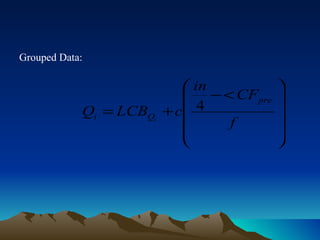
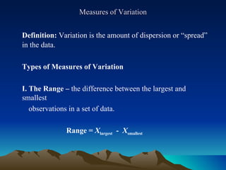
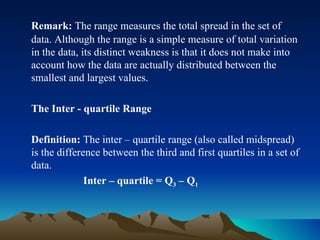
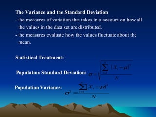
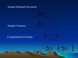
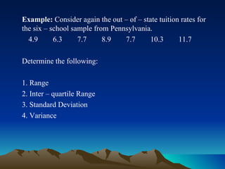
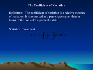
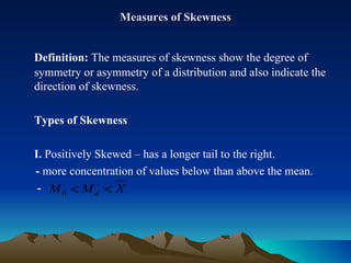
This document defines and describes various measures of central tendency and variation that are used to summarize and describe sets of data. It discusses the mean, median, mode, midrange, percentiles, quartiles, range, variance, standard deviation, interquartile range, coefficient of variation, measures of skewness and kurtosis. Examples are provided to demonstrate how to compute and interpret these statistical measures.

1. Descriptions of Data Measures of Central Tendency Definition: A Measure of Central Tendency has been defined as a statistic calculated from a set of observations or scores and designed to typify or represent that series. It is also defined as the tendency of the same observations or cases to cluster about a point, with either to an absolute value or to a frequency of occurrence; usually but not necessarily, about midway between the extreme high and the extreme low values in the distribution.

2. Measures of Central Tendency The Mean Definition: The arithmetic mean or simply the mean is the average of a group of measures. Characteristics of the mean 1. The arithmetic mean, or simply mean is the center of gravity or balance point of a group of measures. 2. The mean is easily affected by a change in the magnitude of any of the measures.

3. Characteristics of the Mean 3. The mean is the most reliable measure of central tendency because it is always the center of gravity of any group of measures. Uses of the Mean Compute the mean when 1. the mean of a group of measures is needed. 2. the center of gravity or balanced point of a group of measures is wanted. 3. every measure should have an effect upon the measure of central tendency.

4. Uses of the Mean Compute the mean when 4. the most reliable measure of central tendency is desired. 5. the group from which the mean has been derived is more or less homogeneous and a more realistic mean is desired. For instance, the mean of the measure 11, 12, 13, 50, and 64 is 30 which is very far from any of the measures and therefore not realistic. 6. other statistical measures involving the mean are to be computed. Examples of such measures are the standard deviation, coefficient of correlation, critical ratio, etc..

5. Definition: The arithmetic mean or simply the mean of a data set is the sum of the values divided by the number of values. That is, if X 1 , X 2 , . . . , X N are the individual scores in a population of size N , then the population mean is defined as: Definition: If X 1 , X 2 , . . . , X n are the individual scores in a sample size n, then the sample mean is defined as:

6. Example 1: Find the mean of the following scores: 4, 10, 7, 5, 9,7. Example 2: A sample of n = 6 scores has a mean of M = 40. One new score is added to the sample and the new mean is found to be M = 42. What can you conclude about the value of the new score? Definition: For group data or those which are placed in a frequency distribution table, the mean can be approximated by the following formula:

7. Example: Consider the following frequency distribution table of the 15 graduate behavioral statistics students. Classes Frequency 10 – 19 5 20 – 29 4 30 – 39 3 40 – 49 2 50 – 59 1

8. The Weighted Mean Definition: The Weighted Mean is a variation of the arithmetic mean which assigns weight to the individual scores in a data set. where - the weighted mean - the weight - the individual scores - number of cases

9. Example: Suppose we have determined the digit span for a brief time period) in thirty - seven – 4 year – olds. What is the mean digit span for our sample? X f 6 2 5 7 4 17 3 5 2 3 1 2 0 1

10. Example: Consider the following item in a questionnaire . Do you agree that RH bill be implemented? Please check your attitude. _____ Strongly agree _____ Agree _____ Fairly agree _____ Disagree _____ Strongly disagree Suppose 10 individuals were asked to answer the preceding question and the following responses are obtained: 3 - Strongly Agree, 4 – Agree, 2 – Disagree, and 1 – Strongly disagree. What is the average numerical response and its categorical equivalent?

11. Note: Consider the following Hypothetical Mean Range for a 5 point scale categorical responses: 4.20 - 5.00 - Strongly Agree 3.40 - 4.19 - Agree 2.60 - 3.39 - Fairly Agree 1.80 - 2.59 - Disagree 1.00 - 1.79 - Strongly Disagree

12. The Median Definition: The median is the middle most value in an ordered sequence of data. Remark: The median is unaffected by any extreme observations in a set of data and hence, whenever an extreme observation is present, it is appropriate to use the median rather than the mean to describe a set of data. Statistical Treatment: For an even number of observations:

13. For an odd number of observations: Example: A manufacturer of flashlight batteries took a sample of 13 from a day’s production and burned them continuously until they failed. The number of hours they burned were 342 426 317 545 264 451 1049 631 512 266 492 562 298. Determine the median.

14. Example: The following data are the amount of calories in a 30 – gram serving for a random sample of 10 types of fresh – baked chocolate chip cookies. _______________________________________________ Product Calories _______________________________________________ Hillary Rodham Clinton’s 153 Original Nestle Toll House 152 Mrs. Fields 146 Stop and Shop 138 Duncan Hines 130 David’s 146 David’s Chocolate Chunk 149 Great American Cookie Company 138 What is the median amount of calories?

15. The Mode Definition: The mode is the value in a set of data that appears most frequently. It may be obtained from an ordered array. Remark: Unlike the arithmetic mean, the mode is not affected by the occurrence of any extreme values. However, the mode is used only for descriptive purposes because it is more variable from sample to sample than other measures of central tendency. Example: Consider the out – of – state tuition rates for the six – school sample from Pennsylvania. 4.9 6.3 7.7 8.9 7.7 10.3 11.7

16. The Midrange Definition: The midrange is the average of the smallest and largest observations in a set of data. Statistical Treatment: Remark: The midrange is often used as a summary measure both by financial analysts and by weather reporters, since it can provide an adequate, quick, and simple measure to characterize the entire data set – be it a series of daily closing stock prices over a whole year or a series of recorded hourly temperature readings over a whole day.

17. Note: In dealing with data such as daily closing stock prices or hourly temperature readings, an extreme value is not likely to occur. Nevertheless, in most applications, despite its simplicity, the midrange must be used cautiously. Remark: The midrange becomes distorted as a summary measure of central tendency if an outlier is present.

18. Measures of Non-central Location Definition: The measures of non-central location or fractiles are values below which a specified fraction or percentage of a given observation in a data set must fall. Remark: The measures of non-central location are employed particularly when summarizing or describing the properties of large sets of numerical data Types of Fractiles Definition: The percentiles are the 99 score points which divide a distribution of scores into 100 equal parts. Notation: where

19. Ungrouped Data: Formula: observation of the data set placed in array where i = 1, 2, 3, . . . , 99. Grouped Data: Definition: The deciles are the 9 score points which divide the array of observations into 10 equal parts. Ungrouped Data: score where i = 1, 2, 3, . . . , 9

20. Grouped Data: Definition: The quartiles are the 3 score points which divide the array of observations into 4 equal parts. Ungrouped Data: observation of the data set placed in array where i = 1, 2, 3, . . . , 9

21. Grouped Data:

22. Measures of Variation Definition: Variation is the amount of dispersion or “spread” in the data. Types of Measures of Variation I. The Range – the difference between the largest and smallest observations in a set of data. Range = X largest - X smallest

23. Remark: The range measures the total spread in the set of data. Although the range is a simple measure of total variation in the data, its distinct weakness is that it does not make into account how the data are actually distributed between the smallest and largest values. The Inter - quartile Range Definition: The inter – quartile range (also called midspread) is the difference between the third and first quartiles in a set of data. Inter – quartile = Q 3 – Q 1

24. The Variance and the Standard Deviation - the measures of variation that takes into account on how all the values in the data set are distributed. - the measures evaluate how the values fluctuate about the mean. Statistical Treatment: Population Standard Deviation: Population Variance:

25. Sample Standard Deviation: Sample Variance: Computational Formula:

26. Example: Consider again the out – of – state tuition rates for the six – school sample from Pennsylvania. 4.9 6.3 7.7 8.9 7.7 10.3 11.7 Determine the following: 1. Range 2. Inter – quartile Range 3. Standard Deviation 4. Variance

27. The Coefficient of Variation Definition: The coefficient of variation is a relative measure of variation. It is expressed as a percentage rather than in terms of the units of the particular data. Statistical Treatment:

28. Measures of Skewness Definition: The measures of skewness show the degree of symmetry or asymmetry of a distribution and also indicate the direction of skewness. Types of Skewness I. Positively Skewed – has a longer tail to the right. - more concentration of values below than above the mean. -

29. II. Negatively Skewed – has a longer tail to the left. - more concentration of values above than below the mean. - Pearson’s Coefficient of Skewness - use to determine the direction of skewness. Remark: a) If SK > 0, then the distribution is skewed to the right. b) SK < 0, then the distribution of the data set is skewed to left. c) If SK = 0, then the distribution is symmetric.

30. Example: Consider again the out – of – state tuition rates for the six – school sample from Pennsylvania. 4.9 6.3 7.7 8.9 7.7 10.3 11.7 Determine the direction of skewness of the preceding data. Measures of Kurtosis Definition: The measures of kurtosis show the relative flatness or peakedness of a distribution.

31. Types of Kurtosis I. Platykurtic – a distribution which is relatively flat. II. Mesokurtic – a distribution which is between platykurtic and leptokurtic. III. Leptokurtic – a usually peaked distribution. Coefficient of Kurtosis – use to determine the relative flatness of peakedness of a distribution.

32. Statistical Treatment: Remark: a) Ku = 3, then the distribution is mesokurtic b) Ku > 3, then the distribution is leptokurtic. c) Ku < 3, then the distribution is platykurtic Example: Consider again the out – of – state tuition rates for the six – school sample from Pennsylvania. 4.9 6.3 7.7 8.9 7.7 10.3 11.7 Determine the direction of skewness of the preceding data.