The document discusses correlational research methods and statistics, explaining how correlation coefficients measure relationships between variables and allow predictions. It covers the types of relationships (positive, negative, curvilinear), graphical representation through scatterplots, and critical considerations in interpreting correlations such as causality and the third-variable problem. The document also emphasizes the limitations of correlational data, including misinterpretations related to assumed causality and directionality.

1. Reference/Article
Module 18: Correlational Research
Magnitude, Scatterplots, and Types of Relationships
Magnitude
Scatterplots
Positive Relationships
Negative Relationships
No Relationship
Curvilinear Relationships
Misinterpreting Correlations
The Assumptions of Causality and Directionality
The Third-Variable Problem
Restrictive Range
Curvilinear Relationships
Prediction and Correlation
Review of Key Terms
Module Exercises
Critical Thinking Check Answers
Module 19: Correlation Coefficients
The Pearson Product-Moment Correlation Coefficient: What It
Is and What It Does
Calculating the Pearson Product-Moment Correlation
Interpreting the Pearson Product-Moment Correlation
Alternative Correlation Coefficients
Review of Key Terms
Module Exercises
Critical Thinking Check Answers
Module 20: Advanced Correlational Techniques: Regression
Analysis
Regression Lines
Calculating the Slope and y-intercept
Prediction and Regression
Multiple Regression Analysis

2. Review of Key Terms
Module Exercises
Critical Thinking Check Answers
Chapter 9 Summary and Review
Chapter 9 Statistical Software Resources
In this chapter, we discuss correlational research methods and
correlational statistics. As a research method, correlational
designs allow us to describe the relationship between two
measured variables. A correlation coefficient aids us by
assigning a numerical value to the observed relationship. We
begin with a discussion of how to conduct correlational
research, the magnitude and the direction of correlations, and
graphical representations of correlations. We then turn to
special considerations when interpreting correlations, how to
use correlations for predictive purposes, and how to calculate
correlation coefficients. Lastly, we will discuss an advanced
correlational technique, regression analysis.
MODULE 18
Correlational Research
Learning Objectives
•Describe the difference between strong, moderate, and weak
correlation coefficients.
•Draw and interpret scatterplots.
•Explain negative, positive, curvilinear, and no relationship
between variables.
•Explain how assuming causality and directionality, the third-
variable problem, restrictive ranges, and curvilinear
relationships can be problematic when interpreting correlation
coefficients.
•Explain how correlations allow us to make predictions.
When conducting correlational studies, researchers determine
whether two naturally occurring variables (for example, height
and weight, or smoking and cancer) are related to each other.
Such studies assess whether the variables are “co-related” in

3. some way—do people who are taller tend to weigh more, or do
those who smoke tend to have a higher incidence of cancer? As
we saw in Chapter 1, the correlational method is a type of
nonexperimental method that describes the relationship between
two measured variables. In addition to describing a relationship,
correlations also allow us to make predictions from one variable
to another. If two variables are correlated, we can predict from
one variable to the other with a certain degree of accuracy. For
example, knowing that height and weight are correlated would
allow us to estimate, within a certain range, an individual's
weight based on knowing that person's height.
Correlational studies are conducted for a variety of reasons.
Sometimes it is impractical or ethically impossible to do an
experimental study. For example, it would be unethical to
manipulate smoking and assess whether it caused cancer in
humans. How would you, as a subject in an experiment, like to
be randomly assigned to the smoking condition and be told that
you had to smoke a pack of cigarettes a day? Obviously, this is
not a viable experiment, so one means of assessing the
relationship between smoking and cancer is through
correlational studies. In this type of study, we can examine
people who have already chosen to smoke and assess the degree
of relationship between smoking and cancer.
Magnitude, Scatterplots, and Types of Relationships
Correlations vary in their magnitude—the strength of the
relationship. Sometimes there is no relationship between
variables, or the relationship may be weak; other relationships
are moderate or strong. Correlations can also be represented
graphically, in a scatterplot or scattergram. In addition,
relationships are of different types—positive, negative, none, or
curvilinear.
magnitude An indication of the strength of the relationship
between two variables.
Magnitude
The magnitude or strength of a relationship is determined by the
correlation coefficient describing the relationship. A correlation

4. coefficient is a measure of the degree of relationship between
two variables and can vary between − 1.00 and +1.00. The
stronger the relationship between the variables, the closer the
coefficient will be to either −1.00 or +1.00. The weaker the
relationship between the variables, the closer the coefficient
will be to .00. We typically discuss correlation coefficients as
assessing a strong, moderate, or weak relationship, or no
relationship. Table 18.1 provides general guidelines for
assessing the magnitude of a relationship, but these do not
necessarily hold for all variables and all relationships.
correlation coefficient A measure of the degree of relationship
between two sets of scores. It can vary between −1.00 and
+1.00.
A correlation of either −1.00 or +1.00 indicates a perfect
correlation—the strongest relationship you can have. For
example, if height and weight were perfectly correlated (+1.00)
in a group of 20 people, this would mean that the person with
the highest weight would also be the tallest person, the person
with the second-highest weight would be the second-tallest
person, and so on down the line. In addition, in a perfect
relationship, each individual's score on one variable goes
perfectly with his or her score on the other variable, meaning,
for example, that for every increase (decrease) in height of 1
inch, there is a corresponding increase (decrease) in weight of
10 pounds. If height and weight had a perfect negative
correlation (−1.00), this would mean that the person with the
highest weight would be the shortest, the person with the
second-highest weight would be the second shortest, and so on,
and that height and weight increased (decreased) by a set
amount for each individual. It is very unlikely that you will ever
observe a perfect correlation between two variables, but you
may observe some very strong relationships between variables
(+.70−.99). Whereas a correlation coefficient of ±1.00
represents a perfect relationship, a correlation of .00 indicates
no relationship between the variables.
TABLE 18.1 Estimates for weak, moderate, and strong

5. correlation coefficients
correlation coefficient
strength of relationship
±.70−1.00
Strong
±.30−.69
Moderate
±.00−.29
None (.00) to Weak
Scatterplots
A scatterplot or scattergram, a figure showing the relationship
between two variables, graphically represents a correlation
coefficient. Figure 18.1 presents a scatterplot of the height and
weight relationship for 20 adults.
scatterplot A figure that graphically represents the relationship
between two variables.
In a scatterplot, two measurements are represented for each
subject by the placement of a marker. In Figure 18.1, the
horizontal x-axis shows the subject's weight and the vertical y-
axis shows height. The two variables could be reversed on the
axes, and it would make no difference in the scatterplot. This
scatterplot shows an upward trend, and the points cluster in a
linear fashion. The stronger the correlation, the more tightly the
data points cluster around an imaginary line through their
center. When there is a perfect correlation (±1.00), the data
points all fall on a straight line. In general, a scatterplot may
show four basic patterns: a positive relationship, a negative
relationship, no relationship, or a curvilinear relationship.
Positive Relationships
The relationship represented in Figure 18.2a shows a positive
correlation, one in which the two variables move in the same
direction: An increase in one variable is related to an increase
in the other, and a decrease in one is related to a decrease in the
other. Notice that this scatterplot is similar to the one in Figure
18.1. The majority of the data points fall along an upward angle
(from the lower left corner to the upper right corner). In this

6. example, a person who scored low on one variable also scored
low on the other; an individual with a mediocre score on one
variable had a mediocre score on the other; and those who
scored high on one variable also scored high on the other. In
other words, an increase (decrease) in one variable is
accompanied by an increase (decrease) in the other variable—as
variable x increases (or decreases), variable y does the same. If
the data in Figure 18.2a represented height and weight
measurements, we could say that those who are taller also tend
to weigh more, whereas those who are shorter tend to weigh
less.
positive correlation A relationship between two variables in
which the variables move together—an increase in one is related
to an increase in the other, and a decrease in one is related to a
decrease in the other.
FIGURE 18.1 Scatterplot for height and weightFIGURE
18.2Possible types of correlational relationships:
(a)positive;
(b)negative;
(c)none;
(d)curvilinear
Notice also that the relationship is linear: We could draw a
straight line representing the relationship between the variables,
and the data points would all fall fairly close to that line.
Negative Relationships
Figure 18.2b represents a negative relationship between two
variables. Notice that in this scatterplot the data points extend
from the upper left to the lower right. This negative
correlation indicates that an increase in one variable is
accompanied by a decrease in the other variable. This represents
an inverse relationship: The more of variable x that we have,
the less we have of variable y. Assume that this scatterplot
represents the relationship between age and eyesight. As age
increases, the ability to see clearly tends to decrease—a
negative relationship.

7. negative correlation An inverse relationship between two
variables in which an increase in one variable is related to a
decrease in the other, and vice versa.
No Relationship
As shown in Figure 18.2c, it is also possible to observe no
relationship between two variables. In this scatterplot, the data
points are scattered in a random fashion. As you would expect,
the correlation coefficient for these data is very close to zero
(−.09).
Curvilinear Relationships
A correlation of zero indicates no relationship between two
variables. However, it is also possible for a correlation of zero
to indicate a curvilinear relationship, illustrated in Figure
18.2d. Imagine that this graph represents the relationship
between psychological arousal (the x-axis) and performance
(the y-axis). Individuals perform better when they are
moderately aroused than when arousal is either very low or very
high. The correlation for these data is also very close to zero
(−.05). Think about why this would be so. The strong positive
relationship depicted in the left half of the graph essentially
cancels out the strong negative relationship in the right half of
the graph. Although the correlation coefficient is very low, we
would not conclude that there is no relationship between the
two variables. As the figure shows, the variables are very
strongly related to each other in a curvilinear manner—the
points are tightly clustered in an inverted U shape.
Correlation coefficients only tell us about linear relationships.
Thus, even though there is a strong relationship between the two
variables in Figure 18.2d, the correlation coefficient does not
indicate this because the relationship is curvilinear. For this
reason, it is important to examine a scatterplot of the data in
addition to calculating a correlation coefficient. Alternative
statistics (beyond the scope of this text) can be used to assess
the degree of curvilinear relationship between two variables.
TYPES OF RELATIONSHIPS

8. RELATIONSHIP TYPE
Positive
Negative
None
Curvilinear
Description of Relationship
Variables increase and decrease together
As one variable increases, the other decreases—an inverse
relationship
Variables are unrelated and do not move together in any way
Variables increase together up to a point and then as one
continues to increase, the other decreases
Description of Scatterplot
Data points are clustered in a linear pattern extending from
lower left to upper right
Data points are clustered in a linear pattern extending from
upper left to lower right
There is no pattern to the data points—they are scattered all
over the graph
Data points are clustered in a curved linear pattern forming a U
shape or an inverted U shape
Example of Variables Related in This Manner
Smoking and cancer
Mountain elevation and temperature
Intelligence level and weight
Memory and age
1.Which of the following correlation coefficients represents the
weakest relationship between two variables?
− .59
+ .10
− 1.00
+ .76
2.Explain why a correlation coefficient of .00 or close to .00
may not mean that there is no relationship between the

9. variables.
3.Draw a scatterplot representing a strong negative correlation
between depression and self-esteem. Make sure you label the
axes correctly.
Misinterpreting Correlations
Correlational data are frequently misinterpreted, especially
when presented by newspaper reporters, talk-show hosts, or
television newscasters. Here we discuss some of the most
common problems in interpreting correlations. Remember, a
correlation simply indicates that there is a weak, moderate, or
strong relationship (either positive or negative), or no
relationship, between two variables.
The Assumptions of Causality and Directionality
The most common error made when interpreting correlations is
assuming that the relationship observed is causal in nature—that
a change in variable A causes a change in variable B.
Correlations simply identify relationships—they do not indicate
causality. For example, I recently saw a commercial on
television sponsored by an organization promoting literacy. The
statement was made at the beginning of the commercial that a
strong positive correlation has been observed between illiteracy
and drug use in high school students (those high on the
illiteracy variable also tended to be high on the drug-use
variable). The commercial concluded with a statement like
“Let's stop drug use in high school students by making sure they
can all read.” Can you see the flaw in this conclusion? The
commercial did not air for very long, and I suspect someone
pointed out the error in the conclusion.
This commercial made the error of assuming causality and also
the error of assuming directionality. Causality refers to the
assumption that the correlation indicates a causal relationship
between two variables, whereas directionality refers to the
inference made with respect to the direction of a causal
relationship between two variables. For example, the
commercial assumed that illiteracy was causing drug use; it
claimed that if illiteracy were lowered, then drug use would be

10. lowered also. As previously discussed, a correlation between
two variables indicates only that they are related—they move
together. Although it is possible that one variable causes
changes in the other, you cannot draw this conclusion from
correlational data.
causality The assumption that a correlation indicates a causal
relationship between the two variables.
directionality The inference made with respect to the direction
of a relationship between two variables.
Research on smoking and cancer illustrates this limitation of
correlational data. For research with humans, we have only
correlational data indicating a strong positive correlation
between smoking and cancer. Because these data are
correlational, we cannot conclude that there is a causal
relationship. In this situation, it is probable that the relationship
is causal. However, based solely on correlational data, we
cannot conclude that it is causal, nor can we assume the
direction of the relationship. For example, the tobacco industry
could argue that, yes, there is a correlation between smoking
and cancer, but maybe cancer causes smoking—maybe those
individuals predisposed to cancer are more attracted to smoking
cigarettes. Experimental data based on research with laboratory
animals do indicate that smoking causes cancer. The tobacco
industry, however, frequently denied that this research was
applicable to humans and for years continued to insist that no
research had produced evidence of a causal link between
smoking and cancer in humans.
As a further example, research on self-esteem and success also
illustrates the limitations of correlational data. In the pop
psychology literature there are hundreds of books and programs
promoting the idea that there is a causal link between self-
esteem and success. Schools, businesses, and government
offices have implemented programs that offer praise and
complements to their students and employees in the hope of
raising self-esteem and in turn, raising the success of the
students and employees. The problem with this is that the

11. relationship between self-esteem and success is correlational.
However, people misinterpret these claims and make the errors
of assuming causality and directionality (i.e., high self-esteem
causes success). For example, with respect to success in school,
although self-esteem is positively associated with school
success, it appears that better school performance contributes to
high self-esteem, not the reverse (Mercer, 2010, Baumeister et
al., 2003). In other words, focusing on the self-esteem part of
the relationship will likely do little to raise school performance.
A classic example of the assumption of causality and
directionality with correlational data occurred when researchers
observed a strong negative correlation between eye movement
patterns and reading ability in children. Poor readers tended to
make more erratic eye movements, more movements from right
to left, and more stops per line of text. Based on this
correlation, some researchers assumed causality and
directionality: They assumed that poor oculomotor skills caused
poor reading and proposed programs for “eye movement
training.” Many elementary school students who were poor
readers spent time in such training, supposedly developing
oculomotor skills in the hope that this would improve their
reading ability. Experimental research later provided evidence
that the relationship between eye movement patterns and
reading ability is indeed causal but that the direction of the
relationship is the reverse—poor reading causes more erratic
eye movements! Children who are having trouble reading need
to go back over the information more and stop and think about
it more. When children improve their reading skills (improve
recognition and comprehension), their eye movements become
smoother (Olson & Forsberg, 1993). Because of the errors of
assuming causality and directionality, many children never
received the appropriate training to improve their reading
ability.
The Third-Variable Problem
When interpreting a correlation, it is also important to
remember that although the correlation between the variables

12. may be very strong, it may also be that the relationship is the
result of some third variable that influences both of the
measured variables. The third-variable problem results when a
correlation between two variables is dependent on another
(third) variable.
third-variable problem The problem of a correlation between
two variables being dependent on another (third) variable.
A good example of the third-variable problem is a well-cited
study conducted by social scientists and physicians in Taiwan
(Li, 1975). The researchers attempted to identify the variables
that best predicted the use of birth control—a question of
interest to the researchers because of overpopulation problems
in Taiwan. They collected data on various behavioral and
environmental variables and found that the variable most
strongly correlated with contraceptive use was the number of
electrical appliances (yes, electrical appliances—stereos, DVD
players, televisions, and so on) in the home. If we take this
correlation at face value, it means that individuals with more
electrical appliances tend to use contraceptives more, whereas
those with fewer electrical appliances tend to use contraceptives
less.
It should be obvious to you that this is not a causal relationship
(buying electrical appliances does not cause individuals to use
birth control, nor does using birth control cause individuals to
buy electrical appliances). Thus, we probably do not have to
worry about people assuming either causality or directionality
when interpreting this correlation. The problem here is that of a
third variable. In other words, the relationship between
electrical appliances and contraceptive use is not really a
meaningful relationship—other variables are tying these two
together. Can you think of other dimensions on which
individuals who use contraceptives and have a large number of
appliances might be similar? If you thought of education, you
are beginning to understand what is meant by third variables.
Individuals with a higher education level tend to be better
informed about contraceptives and also tend to have a higher

13. socioeconomic status (they get better-paying jobs). The higher
socioeconomic status would allow them to buy more “things,”
including electrical appliances.
It is possible statistically to determine the effects of a third
variable by using a correlational procedure known as partial
correlation. This technique involves measuring all three
variables and then statistically removing the effect of the third
variable from the correlation of the remaining two variables. If
the third variable (in this case, education) is responsible for the
relationship between electrical appliances and contraceptive
use, then the correlation should disappear when the effect of
education is removed, or partialed out.
partial correlation
A correlational technique that involves measuring three
variables and then statistically removing the effect of the third
variable from the correlation of the remaining two variables.
Restrictive Range
The idea behind measuring a correlation is that we assess the
degree of relationship between two variables. Variables, by
definition, must vary. When a variable is truncated, we say that
it has a restrictive range—the variable does not vary enough.
Look at Figure 18.3a, which represents a scatterplot of SAT
scores and college GPAs for a group of students. SAT scores
and GPAs are positively correlated. Neither of these variables is
restricted in range (SAT scores vary from 400 to 1,600 and
GPAs vary from 1.5 to 4.0), so we have the opportunity to
observe a relationship between the variables. Now look
at Figure 18.3b, which represents the correlation between the
same two variables, except that here we have restricted the
range on the SAT variable to those who scored between 1,000
and 1,150. The variable has been restricted or truncated and
does not “vary” very much. As a result, the opportunity to
observe a correlation has been diminished. Even if there were a
strong relationship between these variables, we could not
observe it because of the restricted range of one of the
variables. Thus, when interpreting and using correlations,

14. beware of variables with restricted ranges.
restrictive range A variable that is truncated and does not vary
enough.
FIGURE 18.3 Restricted range and correlation
Curvilinear Relationships
Curvilinear relationships and the problems in interpreting them
were discussed earlier in the module. Remember, correlations
are a measure of linear relationships. When a curvilinear
relationship is present, a correlation coefficient does not
adequately indicate the degree of relationship between the
variables. If necessary, look back over the previous section on
curvilinear relationships to refresh your memory concerning
them.
MISINTERPRETING CORRELATIONS
TYPES OF MISINTERPRETATIONS
Causality and Directionality
Third Variable
Restrictive Range
Curvilinear Relationship
Description of Misinterpretation
Assuming the correlation is causal and that one variable causes
changes in the other
Other variables are responsible for the observed correlation
One or more of the variables is truncated or restricted and the
opportunity to observe a relationship is minimized
The curved nature of the relationship decreases the observed
correlation coefficient
Examples
Assuming that smoking causes cancer or that illiteracy causes
drug abuse because a correlation has been observed
Finding a strong positive relationship between birth control and
number of electrical appliances
If SAT scores are restricted (limited in range), the correlation
between SAT and GPA appears to decrease

15. As arousal increases, performance increases up to a point; as
arousal continues to increase, performance decreases
1.I have recently observed a strong negative correlation between
depression and self-esteem. Explain what this means. Make sure
you avoid the misinterpretations described here.
2.General State University recently investigated the relationship
between SAT scores and GPAs (at graduation) for its senior
class. It was surprised to find a weak correlation between these
two variables. The university knows it has a grade inflation
problem (the whole senior class graduated with GPAs of 3.0 or
higher), but it is unsure how this might help account for the low
correlation observed. Can you explain?
Prediction and Correlation
Correlation coefficients not only describe the relationship
between variables; they also allow us to make predictions from
one variable to another. Correlations between variables indicate
that when one variable is present at a certain level, the other
also tends to be present at a certain level. Notice the wording
used. The statement is qualified by the use of the phrase “tends
to.” We are not saying that a prediction is guaranteed, nor that
the relationship is causal—but simply that the variables seem to
occur together at specific levels. Think about some of the
examples used previously in this module. Height and weight are
positively correlated. One is not causing the other, nor can we
predict exactly what an individual's weight will be based on
height (or vice versa). But because the two variables are
correlated, we can predict with a certain degree of accuracy
what an individual's approximate weight might be if we know
the person's height.
Let's take another example. We have noted a correlation
between SAT scores and college freshman GPAs. Think about
what the purpose of the SAT is. College admissions committees
use the test as part of the admissions procedure. Why? They use
it because there is a positive correlation between SAT scores
and college GPAs. Individuals who score high on the SAT tend

16. to have higher college freshman GPAs; those who score lower
on the SAT tend to have lower college freshman GPAs. This
means that knowing students' SAT scores can help predict, with
a certain degree of accuracy, their freshman GPA and thus their
potential for success in college. At this point, some of you are
probably saying, “But that isn't true for me—I scored poorly (or
very well) on the SAT and my GPA is great (or not so good).”
Statistics only tell us what the trend is for most people in the
population or sample. There will always be outliers—the few
individuals who do not fit the trend. Most people, however, are
going to fit the pattern.
Think about another example. We know there is a strong
positive correlation between smoking and cancer, but you may
know someone who has smoked for 30 or 40 years and does not
have cancer or any other health problems. Does this one
individual negate the fact that there is a strong relationship
between smoking and cancer? No. To claim that it does would
be a classic person-who argument—arguing that a well-
established statistical trend is invalid because we know a
“person who” went against the trend (Stanovich, 2007). A
counterexample does not change the fact of a strong statistical
relationship between the variables, and that you are increasing
your chance of getting cancer if you smoke. Because of the
correlation between the variables, we can predict (with a fairly
high degree of accuracy) who might get cancer based on
knowing a person's smoking history.
person-who argument Arguing that a well-established statistical
trend is invalid because we know a “person who” went against
the trend.
REVIEW OF KEY TERMS
causality (p. 317)
correlation coefficient (p. 313)
directionality (p. 317)
magnitude (p. 313)
negative correlation (p. 315)
partial correlation (p. 319)

17. person-who argument (p. 322)
positive correlation (p. 314)
restrictive range (p. 319)
scatterplot (p. 314)
third-variable problem (p. 319)
MODULE EXERCISES
(Answers to odd-numbered questions appear in Appendix B.)
1.A health club recently conducted a study of its members and
found a positive relationship between exercise and health. It
claimed that the correlation coefficient between the variables of
exercise and health was +1.25. What is wrong with this
statement? In addition, the club stated that this proved that an
increase in exercise increases health. What is wrong with this
statement?
2.Draw a scatterplot indicating a strong negative relationship
between the variables of income and mental illness. Be sure to
label the axes correctly.
3.Explain why the correlation coefficient for a curvilinear
relationship would be close to .00.
4.Explain why the misinterpretations of causality and
directionality always occur together.
5.We have mentioned several times that there is a fairly strong
positive correlation between SAT scores and freshman GPAs.
The admissions process for graduate school is based on a
similar test, the GRE, which also has a potential 400 to 1,600
total point range. If graduate schools do not accept anyone who
scores below 1,000 and if a GPA below 3.00 represents failing
work in graduate school, what would we expect the correlation
between GRE scores and graduate school GPAs to be like in
comparison to that between SAT scores and college GPAs? Why
would we expect this?
6.Why is the correlational method a predictive method? In other
words, how does establishing that two variables are correlated
allow us to make predictions?
CRITICAL THINKING CHECK ANSWERS
Critical Thinking Check 18.1

18. 1.+.10
2.A correlation coefficient of .00 or close to .00 may indicate
no relationship or a weak relationship. However, if the
relationship is curvilinear, the correlation coefficient could also
be .00 or close to it. In this case, there would be a relationship
between the two variables, but because of the curvilinear nature
of the relationship the correlation coefficient would not truly
represent the strength of the relationship.
3.
Critical Thinking Check 18.2
1.A strong negative correlation between depression and self-
esteem means that individuals who are more depressed also tend
to have lower self-esteem, whereas individuals who are less
depressed tend to have higher self-esteem. It does not mean that
one variable causes changes in the other, but simply that the
variables tend to move together in a certain manner.
2.General State University observed such a low correlation
between GPAs and SAT scores because of a restrictive range on
the GPA variable. Because of grade inflation, the whole senior
class graduated with a GPA of 3.0 or higher. This restriction on
one of the variables lessens the opportunity to observe a
correlation.
MODULE 19
Correlation Coefficients
Learning Objectives
•Describe when it would be appropriate to use the Pearson
product-moment correlation coefficient, the Spearman rank-
order correlation coefficient, the point-biserial correlation
coefficient, and the phi coefficient.
•Calculate of the Pearson product-moment correlation
coefficient for two variables.
•Determine and explain r2 for a correlation coefficient.
Now that you understand how to interpret a correlation

19. coefficient, let's turn to the actual calculation of correlation
coefficients. The type of correlation coefficient used depends on
the type of data (nominal, ordinal, interval, or ratio) that were
collected.
The Pearson Product-Moment Correlation Coefficient: What It
Is and What It Does
The most commonly used correlation coefficient is the Pearson
product-moment correlation coefficient, usually referred to
as Pearson's r(r is the statistical notation we use to report
correlation coefficients). Pearson's r is used for data measured
on an interval or ratio scale of measurement. Refer back
to Figure 18.1 in the previous module, which presents a
scatterplot of height and weight data for 20 individuals.
Because height and weight are both measured on a ratio scale,
Pearson's r would be applicable to these data.
Pearson product-moment correlation coefficient (Pearson's
r) The most commonly used correlation coefficient. It is used
when both variables are measured on an interval or ratio scale.
The development of this correlation coefficient is typically
credited to Karl Pearson (hence the name), who published his
formula for calculating r in 1895. Actually, Francis Edgeworth
published a similar formula for calculating r in 1892. Not
realizing the significance of his work, however, Edgeworth
embedded the formula in a statistical paper that was very
difficult to follow, and it was not noted until years later. Thus,
although Edgeworth had published the formula three years
earlier, Pearson received the recognition (Cowles, 1989).
Calculating the Pearson Product-Moment Correlation
Table 19.1 presents the raw scores from which the scatterplot
in Figure 18.1 (in the previous module) was derived, along with
the mean and standard deviation for each distribution. Height is
presented in inches and weight in pounds. Let's use these data to
demonstrate the calculation of Pearson's r.
TABLE 19.1 Height and weight data for 20 individuals
WEIGHT (IN POUNDS)
HEIGHT (IN INCHES)

20. 100
60
120
61
105
63
115
63
119
65
134
65
129
66
143
67
151
65
163
67
160
68
176
69
165
70
181
72
192
76
208
75
200
77
152
68

21. 134
66
138
65
μ = 149.25
μ = 67.4
σ = 30.42
σ = 4.57
To calculate Pearson's r, we need to somehow convert the raw
scores on the two different variables into the same unit of
measurement. This should sound familiar to you from an earlier
module. You may remember from Module 6 that we
used z scores to convert data measured on different scales to
standard scores measured on the same scale (a z score simply
represents the number of standard deviation units a raw score is
above or below the mean). Thus, high raw scores will always be
above the mean and have positive z scores, and low raw scores
will be below the mean and thus have negative z scores.
Think about what will happen if we convert our raw scores on
height and weight over to z scores. If the correlation is strong
and positive, we should find that positive z scores on one
variable go with positive z scores on the other variable and
negative z scores on one variable go with negative z scores on
the other variable.
After calculating z scores, the next step in calculating
Pearson's r is to calculate what is called a cross-product—
the z score on one variable multiplied by the z score on the
other variable. This is also sometimes referred to as a cross-
product of z scores. Once again, think about what will happen if
both z scores used to calculate the cross-product are positive—
the cross-product will be positive. What if both z scores are
negative? Once again, the cross-product will be positive (a
negative number multiplied by a negative number results in a
positive number). If we summed all of these positive cross-
products and divided by the total number of cases (to obtain the
average of the cross-products), we would end up with a large

22. positive correlation coefficient.
What if we found that, when we converted our raw scores
to z scores, positive z scores on one variable went with
negative z scores on the other variable? These cross-products
would be negative and when averaged (that is, summed and
divided by the total number of cases) would result in a large
negative correlation coefficient.
Lastly, imagine what would happen when there is no linear
relationship between the variables being measured. In other
words, some individuals who score high on one variable also
score high on the other, and some individuals who score low on
one variable score low on the other. Each of the previous
situations results in positive cross-products. However, you also
find that some individuals with high scores on one variable have
low scores on the other variable, and vice versa. This would
result in negative cross-products. When all of the cross-products
are summed and divided by the total number of cases, the
positive and negative cross-products would essentially cancel
each other out, and the result would be a correlation coefficient
close to zero.
TABLE 19.2 Calculating the Pearson correlation coefficient
X
(WEIGHT IN POUNDS)
Y
(HEIGHT IN INCHES)
Zx
Zy
ZxZy
100
60
−1.62
−1.62
2.62
120
61
−0.96

23. − 1.40
1.34
105
63
−1.45
−0.96
1.39
115
63
−1.13
−0.96
1.08
119
65
−0.99
−0.53
0.52
134
65
−0.50
−0.53
0.27
129
66
−0.67
−0.31
0.21
143
67
−0.21
−0.09
0.02
151
65
0.06
−0.53

24. −0.03
163
67
0.45
−0.09
−0.04
160
68
0.35
0.13
0.05
176
69
0.88
0.35
0.31
165
70
0.52
0.57
0.30
181
72
1.04
1.01
1.05
192
76
1.41
1.88
2.65
208
75
1.93
1.66
3.20

25. 200
77
1.67
2.10
3.51
152
68
0.09
0.13
0.01
134
66
−0.50
−0.31
0.16
138
65
−0.37
−0.53
0.20
Σ = +18.82
Now that you have a basic understanding of the logic behind
calculating Pearson's r, let's look at the formula for Pearson's r:
r=ΣZXZYN
where
Σ=the summation ofZx=the z score for variable X for each indivi
dualZY=the z score for variable X for each individual N=the num
ber of individuals in the sample
Thus, we begin by calculating the z scores for X (weight)
and Y (height). This is shown in Table 19.2. Remember, the
formula for a z score is
z=X−μσ
where
X=each individual scoreμ=the population meanσ=the population
standard deviation
The first two columns in Table 19.2 list the height and weight

26. raw scores for the 20 individuals. As a general rule of thumb,
when calculating a correlation coefficient, you should have at
least 10 subjects per variable; with two variables, we need a
minimum of 20 individuals, which we have. Following the raw
scores for variable X (weight) and variable Y(height) are
columns representing ZX, ZY, and ZXZY (the cross-product
of z scores). The cross-products column has been summed (Σ) at
the bottom of the table.
Now, let's use the information from the table to calculate r:
r=ΣZXZYN=18.8220=+.94
Interpreting the Pearson Product-Moment Correlation
The obtained correlation between height and weight for the 20
individuals represented in the table is +.94. Can you interpret
this correlation coefficient? The positive sign tells us that the
variables increase and decrease together. The large magnitude
(close to 1.00) tells us that there is a strong positive
relationship between height and weight. However, we can also
determine whether this correlation coefficient is statistically
significant, as we have done with other statistics. The null
hypothesis (H0) when we are testing a correlation coefficient is
that the true population correlation coefficient is .00—the
variables are not related. The alternative hypothesis (Ha) is that
the observed correlation is not equal to .00—the variables are
related. In order to test the null hypothesis that the population
correlation coefficient is .00, we must consult a table of critical
values for r (the Pearson product-moment correlation
coefficient). Table A.6 in Appendix A shows critical values for
both one- and two-tailed tests of r. A one-tailed test of a
correlation coefficient means that you have predicted the
expected direction of the correlation coefficient, whereas a two-
tailed test means that you have not predicted the direction of the
correlation coefficient.
To use this table, we first need to determine the degrees of
freedom, which for the Pearson product-moment correlation are
equal to N − 2, where N represents the total number of pairs of
observations. Our correlation coefficient of +.94 is based on 20

27. pairs of observations; thus, the degrees of freedom are 20 −
2 = 18. Once the degrees of freedom have been determined, we
can consult the critical values table. For 18 degrees of freedom
and a one-tailed test (the test is one-tailed because we expect a
positive relationship between height and weight) at α = .05,
the rcv is ± .3783. This means that our robt must be that large
or larger in order to be statistically significant at the .05 level.
Because our robt is that large, we would reject H0. In other
words, the observed correlation coefficient is statistically
significant, and we can conclude that those who are taller tend
to weigh significantly more, whereas those who are shorter tend
to weigh significantly less.
Because robt was significant at the .05 level, we should check
for significance at the .025 and .005 levels provided in Table
A.6. Our robt of + .94 is larger than the critical values at all of
the levels of significance provided in Table A.6. In APA
publication format, this would be reported as r(18) = + .94, p <
.005, one-tailed. You can see how to use either Excel, SPSS, or
the TI-84 calculator to calculate Pearson's r in the Statistical
Software Resources section at the end of this chapter.
In addition to interpreting the correlation coefficient, it is
important to calculate the coefficient of determination (r2).
Calculated by squaring the correlation coefficient, the
coefficient of determination is a measure of the proportion of
the variance in one variable that is accounted for by another
variable. In our group of 20 individuals, there is variation in
both the height and weight variables, and some of the variation
in one variable can be accounted for by the other variable. We
could say that the variation in the weights of these 20
individuals can be explained by the variation in their heights.
Some of the variation in their weights, however, cannot be
explained by the variation in height. It might be explained by
other factors such as genetic predisposition, age, fitness level,
or eating habits. The coefficient of determination tells us how
much of the variation in weight is accounted for by the variation
in height. Squaring the obtained correlation coefficient of + .94,

28. we have r2 = .8836. We typically report r2 as a percentage.
Hence, 88.36% of the variance in weight can be accounted for
by the variance in height—a very high coefficient of
determination. Depending on the research area, the coefficient
of determination could be much lower and still be important. It
is up to the researcher to interpret the coefficient of
determination accordingly.
coefficient of determination (r2) A measure of the proportion of
the variance in one variable that is accounted for by another
variable; calculated by squaring the correlation coefficient.
Alternative Correlation Coefficients
As noted previously, the type of correlation coefficient used
depends on the type of data collected in the research study.
Pearson's correlation coefficient is used when both variables are
measured on an interval or ratio scale. Alternative correlation
coefficients can be used with ordinal and nominal scales of
measurement. We will mention three such correlation
coefficients but will not present the formulas because our
coverage of statistics is necessarily selective. All of the
formulas are based on Pearson's formula and can be found in a
more advanced statistics text. Each of these coefficients is
reported on a scale of −1.00 to +1.00. Thus, each is interpreted
in a fashion similar to Pearson's r. Lastly, as with Pearson's r,
the coefficient of determination (r2) can be calculated for each
of these correlation coefficients to determine the proportion of
variance in one variable accounted for by the other variable.
When one or more of the variables is measured on an ordinal
(ranking) scale, the appropriate correlation coefficient
is Spearman's rank-order correlation coefficient. If one of the
variables is interval or ratio in nature, it must be ranked
(converted to an ordinal scale) before you do the calculations. If
one of the variables is measured on a dichotomous (having only
two possible values, such as gender) nominal scale and the other
is measured on an interval or ratio scale, the appropriate
correlation coefficient is the point-biserial correlation
coefficient. Lastly, if both variables are dichotomous and

29. nominal, the phi coefficient is used.
Spearman's rank-order correlation coefficient The correlation
coefficient used when one or more of the variables is measured
on an ordinal (ranking) scale.
point-biserial correlation coefficient The correlation coefficient
used when one of the variables is measured on a dichotomous
nominal scale and the other is measured on an interval or ratio
scale.
phi coefficient The correlation coefficient used when both
measured variables are dichotomous and nominal.
Although both the point-biserial and phi coefficients are used to
calculate correlations with dichotomous nominal variables, you
should refer back to one of the cautions mentioned in the
previous module concerning potential problems when
interpreting correlation coefficients—specifically, the caution
regarding restricted ranges. Clearly, a variable with only two
levels has a restricted range. Can you think about what the
scatterplot for such a correlation would look like? The points
would have to be clustered into columns or groups, depending
on whether one or both of the variables were dichotomous.
CORRELATION COEFFICIENTS
TYPES OF COEFFICIENTS
Pearson
Spearman
Point-Biserial
Phi
Type of Data
Both variables must be interval or ratio
Both variables are ordinal (ranked)
One variable is interval or ratio, and one variable is nominal
and dichotomous
Both variables are nominal and dichotomous
Correlation

30. ±.00−1.0
±.00−1.0
±.00−1.0
±.00−1.0
Reported as r2 Applicable?
Yes
Yes
Yes
Yes
1.Professor Hitch found that the Pearson product-moment
correlation between the height and weight of the 32 students in
her class was +.35. Using Table A.6 in Appendix A, for a one-
tailed test, determine whether this is a significant correlation
coefficient. Determine the coefficient of determination for the
correlation coefficient, and explain what it means.
2.In a recent study, researchers were interested in determining
the relationship between gender and amount of time spent
studying for a group of college students. Which correlation
coefficient should be used to assess this relationship?
REVIEW OF KEY TERMS
coefficient of determination (r2) (p. 328)
Pearson product-moment correlation coefficient (Pearson's
r) (p. 324)
phi coefficient (p. 329)
point-biserial correlation coefficient (p. 329)
Spearman's rank-order correlation coefficient (p. 328)
MODULE EXERCISES
(Answers to odd-numbered questions appear in Appendix B.)
1.Explain when the Pearson product-moment correlation
coefficient should be used.
2.In a study of caffeine and stress, college students indicate
how many cups of coffee they drink per day and their stress
level on a scale of 1 to 10. The data follow:
Number of Cups of Coffee
Stress Level

31. 3
5
2
3
4
3
6
9
5
4
1
2
7
10
3
5
Calculate a Pearson's r to determine the type and strength of the
relationship between caffeine and stress level.
3.How much of the variability in stress scores in exercise 2 is
accounted for by the number of cups of coffee consumed per
day?
4.Given the following data, determine the correlation between
IQ scores and psychology exam scores, between IQ scores and
statistics exam scores, and between psychology exam scores and
statistics exam scores.
Student
IQ Score
Psychology Exam Score
Statistics Exam Score
1
140
48
47
2
98
35

32. 32
3
105
36
38
4
120
43
40
5
119
30
40
6
114
45
43
7
102
37
33
8
112
44
47
9
111
38
46
10
116
46
44
5.Calculate the coefficient of determination for each of the
correlation coefficients in exercise 4, and explain what these
mean.

33. 6.Explain when it would be appropriate to use the phi
coefficient versus the point-biserial coefficient.
7.If one variable is ordinal and the other is interval-ratio, which
correlation coefficient should be used?
CRITICAL THINKING CHECK ANSWERS
Critical Thinking Check 19.1
1.Yes. For a one-tailed test, r(30) = .35, p < .025. The
coefficient of determination (r2) = .1225. This means that
height can explain 12.25% of the variance observed in the
weight of these individuals.
2.In this study, gender is nominal in scale, and the amount of
time spent studying is ratio in scale. Thus, a point-biserial
correlation coefficient would be appropriate.
MODULE 20
Advanced Correlational Techniques: Regression Analysis
Learning Objectives
•Explain what regression analysis is.
•Determine the regression line for two variables.
As we have seen, the correlational procedure allows us to
predict from one variable to another, and the degree of accuracy
with which you can predict depends on the strength of the
correlation. A tool that enables us to predict an individual's
score on one variable based on knowing one or more other
variables is known as regression analysis. For example, imagine
that you are an admissions counselor at a university and you
want to predict how well a prospective student might do at your
school based on both SAT scores and high school GPA. Or
imagine that you work in a human resources office and you
want to predict how well future employees might perform based
on test scores and performance measures. Regression analysis
allows you to make such predictions by developing a regression
equation.
regression analysis A procedure that allows us to predict an
individual's score on one variable based on knowing one or

34. more other variables.
To illustrate regression analysis, let's use the height and weight
data presented in Table 20.1. When we used these data to
calculate Pearson's r (in Module 19), we determined that the
correlation coefficient was +.94. Also, we can see in Figure
18.1 (in Module 18) that there is a linear relationship between
the variables, meaning that a straight line can be drawn through
the data to represent the relationship between the variables.
This regression line is shown in Figure 20.1; it represents the
relationship between height and weight for this group of
individuals.
regression line The best-fitting straight line drawn through the
center of a scatterplot that indicates the relationship between
the variables.
Regression Lines
Regression analysis involves determining the equation for the
best-fitting line for a data set. This equation is based on the
equation for representing a line you may remember from algebra
class: y = mx + b, where m is the slope of the line and b is
the y-intercept (the place where the line crosses the y-axis). For
a linear regression analysis, the formula is essentially the same,
although the symbols differ:
Y′=bX+a
FIGURE 20.1 The relationship between height and weight, with
the regression line indicatedTABLE 20.1 Height and weight
data for 20 individuals
WEIGHT(IN POUNDS)
HEIGHT (IN INCHES)
100
60
120
61
105
63
115
63

35. 119
65
134
65
129
66
143
67
151
65
163
67
160
68
176
69
165
70
181
72
192
76
208
75
200
77
152
68
134
66
138
65
μ = 149.25
μ = 67.4
σ = 30.42
σ = 4.57

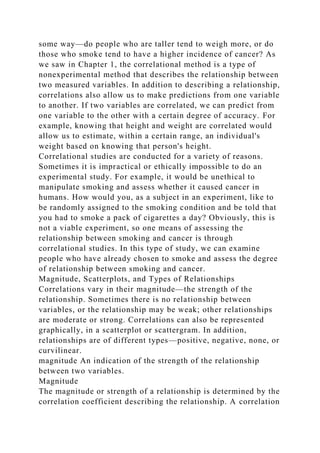
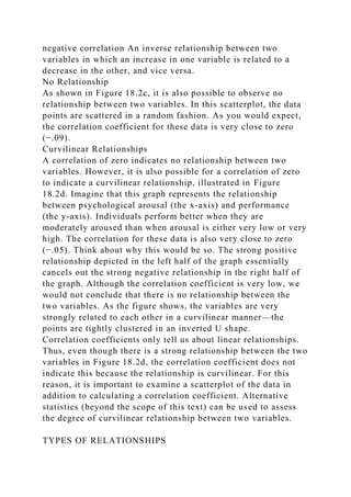
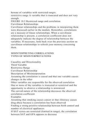
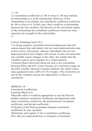
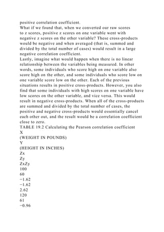
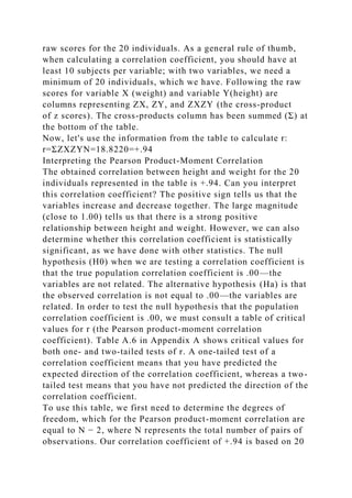
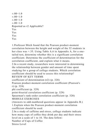
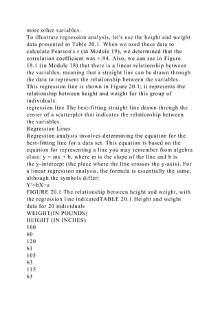
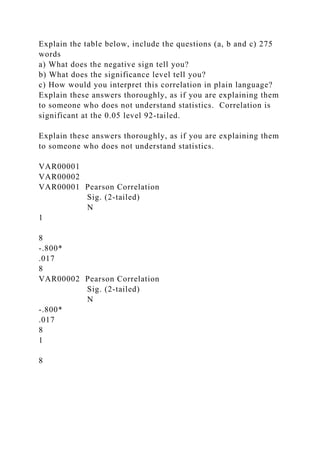
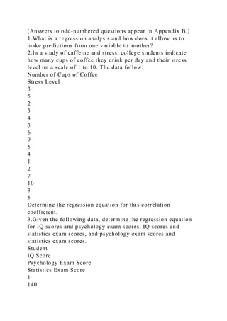
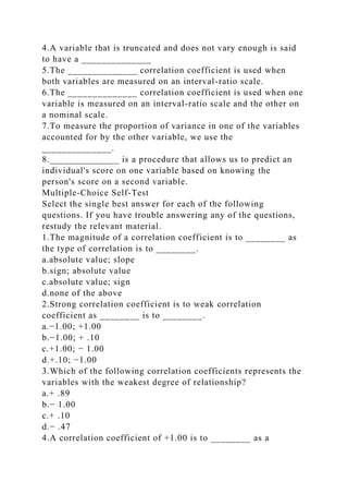
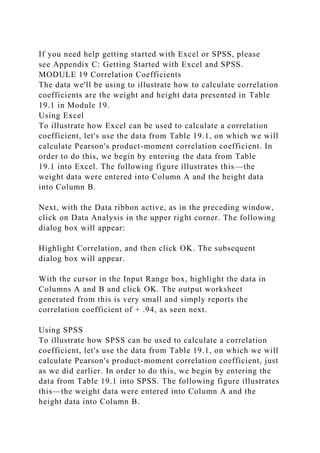
36. where Y' is the predicted value on the Y variable, b is the slope
of the line, X represents an individual's score on the X variable,
and a is the y-intercept.
Using this formula, then, we can predict an individual's
approximate score on variable Y based on that person's score on
variable X. With the height and weight data, for example, we
could predict an individual's approximate height based on
knowing the person's weight. You can picture what we are
talking about by looking at Figure 20.1 Given the regression
line in Figure 20.1, if we know an individual's weight (read
from the x-axis), we can then predict the person's height (by
finding the corresponding value on the y -axis).
Calculating the Slope and y-Intercept
To use the regression line formula, we need to determine
both b and a. Let's begin with the slope (b). The formula for
computing b is
b=r[ σYσX ]
This should look fairly simple to you. We have already
calculated r in the previous module (+ .94) and the standard
deviations (σ) for both height and weight (see Table 20.1).
Using these calculations, we can compute b as follows:
b=.94[ 4.5730.42 ]=.94(0.150)=.141
Now that we have computed b, we can compute a. The formula
for a is
a=Y¯−b(X¯)
Once again, this should look fairly simple, because we have just
calculated b, and Y¯ and X¯ (the means for
the Y and X variables—height and weight, respectively) are
presented in Table 20.1. Using these values in the formula for a,
we have
a=67.40 − 0.141(149.25)=67.40−21.04=46.36
Thus, the regression equation for the line for the data in Figure
20.1 is
Y′(height)=0.141X(weight)+46.36
where 0.141 is the slope and 46.36 is the y-intercept.
Prediction and Regression

37. Now that we have calculated the equation for the regression
line, we can use this line to predict from one variable to
another. For example, if we know that an individual weighs 110
pounds, we can predict the person's height using this equation:
Y′=0.141(110)+46.36=15.51+46.36=61.87 inches
Let's make another prediction using this regression line. If
someone weighs 160 pounds, what would we predict their height
to be? Using the regression equation, this would be
Y′=0.141(160)+46.36=22.561+46.36=68.92 inches
As we can see, determining the regression equation for a set of
data allows us to predict from one variable to the other. The
stronger the relationship between the variables (that is, the
stronger the correlation coefficient), the more accurate the
prediction will be. The calculations for regression analysis
using Excel, SPSS, and the TI-84 calculator are presented in the
Statistical Software Resources section at the end of this chapter.
Multiple Regression Analysis
A more advanced use of regression analysis is known
as multiple regression analysis. Multiple regression analysis
involves combining several predictor variables into a single
regression equation. This is analogous to the factorial ANOVAs
we discussed in Modules 16 and 17, in that we can assess the
effects of multiple predictor variables (rather than a single
predictor variable) on the dependent measure. In our height and
weight example, we attempted to predict an individual's height
based on knowing the person's weight. There might be other
variables we could add to the equation that would increase our
predictive ability. For example, if, in addition to the
individual's weight, we knew the height of the biological
parents, this might increase our ability to accurately predict the
person's height.
When using multiple regression, the predicted value
of Y' represents the linear combination of all the predictor
variables used in the equation. The rationale behind using this
more advanced form of regression analysis is that in the real
world it is unlikely that one variable is affected by only one

38. other variable. In other words, real life involves the interaction
of many variables on other variables. Thus, in order to more
accurately predict variable A, it makes sense to consider all
possible variables that might influence variable A. In terms of
our example, it is doubtful that height is influenced only by
weight. There are many other variables that might help us to
predict height, such as the variable just mentioned—the height
of each biological parent. The calculation of multiple regression
is beyond the scope of this book. For further information on it,
consult a more advanced statistics text.
REGRESSION ANALYSIS
Concept
What It Does
Regression Analysis
A tool that enables one to predict an individual's score on one
variable based on knowing one or more other variables
Regression Line
The equation for the best-fitting line for a data set. The
equation is based on determining the slope and y-intercept for
the best-fitting line and is as follows: Y′ = bX + a, where Y′ is
the predicted value on the Y variable, b is the slope of the
line, X represents an individual's score on the X variable,
and a is the y-intercept
Multiple Regression
A type of regression analysis that involves combining several
predictor variables into a singe regression equation
1.How does determining a best-fitting line help us to predict
from one variable to another?
2.For the example in the text, if an individual's weight was 125
pounds, what would the predicted height be?
REVIEW OF KEY TERMS
regression analysis (p. 331)
regression line (p. 331)
MODULE EXERCISES

39. (Answers to odd-numbered questions appear in Appendix B.)
1.What is a regression analysis and how does it allow us to
make predictions from one variable to another?
2.In a study of caffeine and stress, college students indicate
how many cups of coffee they drink per day and their stress
level on a scale of 1 to 10. The data follow:
Number of Cups of Coffee
Stress Level
3
5
2
3
4
3
6
9
5
4
1
2
7
10
3
5
Determine the regression equation for this correlation
coefficient.
3.Given the following data, determine the regression equation
for IQ scores and psychology exam scores, IQ scores and
statistics exam scores, and psychology exam scores and
statistics exam scores.
Student
IQ Score
Psychology Exam Score
Statistics Exam Score
1
140

40. 48
47
2
98
35
32
3
105
36
38
4
120
43
40
5
119
30
40
6
114
45
43
7
102
37
33
8
112
44
47
9
111
38
46
10
116

41. 46
44
4.Assuming that the regression equation for the relationship
between IQ score and psychology exam score is Y' = .274X + 9,
what would you expect the psychology exam score to be for the
following individuals, given their IQ exam score?
Individual
IQ Score (X)
Psychology Exam Score (Y' )
Tim
118
Tom
98
Tina
107
Tory
103
CRITICAL THINKING CHECK ANSWERS
Critical Thinking Check 20.1
1.The best-fitting line is the line that comes closest to all of the
data points in a scatterplot. Given this line, we can predict from
one variable to another by determining where on the line an
individual's score on one variable lies and then determining
what the score would be on the other variable based on this.
2.If an individual weighed 125 pounds and we used the
regression line determined in this module to predict height, then
Y′=0.141(125)+46.36=17.625+46.36=63.985 inches
CHAPTER NINE SUMMARY AND REVIEW
Correlational Procedures
CHAPTER SUMMARY

42. After reading this chapter, you should have an understanding of
correlational research, which allows researchers to observe
relationships between variables; correlation coefficients, the
statistics that assess that relationship; and regression analysis, a
procedure that allows us to predict from one variable to another.
Correlations vary in type (positive or negative) and magnitude
(weak, moderate, or strong). The pictorial representation of a
correlation is a scatterplot. Scatterplots allow us to see the
relationship, facilitating its interpretation.
When interpreting correlations, several errors are commonly
made. These include assuming causality and directionality, the
third-variable problem, having a restrictive range on one or both
variables, and the problem of assessing a curvilinear
relationship. Knowing that two variables are correlated allows
researchers to make predictions from one variable to another.
Four different correlation coefficients (Pearson's, Spearman's,
point-biserial, and phi) and when each should be used were
discussed. The coefficient of determination was also discussed
with respect to more fully understanding correlation
coefficients. Lastly, regression analysis, which allows us to
predict from one variable to another, was described.
CHAPTER 9 REVIEW EXERCISES
(Answers to exercises appear in Appendix B.)
Fill-in Self-Test
Answer the following questions. If you have trouble answering
any of the questions, restudy the relevant material before going
on to the multiple-choice self-test.
1.A ______________ is a figure that graphically represents the
relationship between two variables.
2.When an increase in one variable is related to a decrease in
the other variable, and vice versa, we have observed an inverse
or ______________ relationship.
3.When we assume that because we have observed a correlation
between two variables, one variable must be causing changes in
the other variable, we have made the errors of ______________
and ______________.

43. 4.A variable that is truncated and does not vary enough is said
to have a ______________
5.The ______________ correlation coefficient is used when
both variables are measured on an interval-ratio scale.
6.The ______________ correlation coefficient is used when one
variable is measured on an interval-ratio scale and the other on
a nominal scale.
7.To measure the proportion of variance in one of the variables
accounted for by the other variable, we use the
______________.
8.______________ is a procedure that allows us to predict an
individual's score on one variable based on knowing the
person's score on a second variable.
Multiple-Choice Self-Test
Select the single best answer for each of the following
questions. If you have trouble answering any of the questions,
restudy the relevant material.
1.The magnitude of a correlation coefficient is to ________ as
the type of correlation is to ________.
a.absolute value; slope
b.sign; absolute value
c.absolute value; sign
d.none of the above
2.Strong correlation coefficient is to weak correlation
coefficient as ________ is to ________.
a.−1.00; +1.00
b.−1.00; + .10
c.+1.00; − 1.00
d.+.10; −1.00
3.Which of the following correlation coefficients represents the
variables with the weakest degree of relationship?
a.+ .89
b.− 1.00
c.+ .10
d.− .47
4.A correlation coefficient of +1.00 is to ________ as a

44. correlation coefficient of −1.00 is to ________.
a.no relationship; weak relationship
b.weak relationship; perfect relationship
c.perfect relationship; perfect relationship
d.perfect relationship; no relationship
5.If the points on a scatterplot are clustered in a pattern that
extends from the upper left to the lower right, this would
suggest that the two variables depicted are
a.normally distributed.
b.positively correlated.
c.regressing toward the average.
d.negatively correlated.
6.We would expect the correlation between height and weight to
be ________, whereas we would expect the correlation between
age in adults and hearing ability to be ________.
a.curvilinear; negative
b.positive; negative
c.negative; positive
d.positive; curvilinear
7.When we argue against a statistical trend based on one case,
we are using a
a.third variable.
b.regression analysis.
c.partial correlation.
d.person-who argument.
8.If a relationship is curvilinear, we would expect the
correlation coefficient to be
a.close to .00.
b.close to + 1.00.
c.close to −1.00.
d.an accurate representation of the strength of the relationship.
9.The ________ is the correlation coefficient that should be
used when both variables are measured on an ordinal scale.
a.Spearman rank-order correlation coefficient
b.coefficient of determination
c.point-biserial correlation coefficient

45. d.Pearson product-moment correlation coefficient
10.Suppose that the correlation between age and hearing ability
for adults is −.65. What proportion (or percentage) of the
variability in hearing ability is accounted for by the relationship
with age?
a.65%
b.35%
c.42%
d.unable to determine
11.Drew is interested in assessing the degree of relationship
between belonging to a Greek organization and number of
alcoholic drinks consumed per week. Drew should use the
________ correlation coefficient to assess this.
a.partial
b.point-biserial
c.phi
d.Pearson product-moment
12.Regression analysis allows us to
a.predict an individual's score on one variable based on
knowing the person's score on another variable.
b.determine the degree of relationship between two interval-
ratio variables.
c.determine the degree of relationship between two nominal
variables.
d.predict an individual's score on one variable based on
knowing that the variable is interval-ratio in scale.
Self-Test Problem
1.Professor Mumblemore wants to determine the degree of
relationship between students' scores on their first and second
exams in his chemistry class. The scores received by students
on the first and second exams follow:
Student
Score on Exam 1
Score on Exam 2
Sarah
81

46. 87
Ned
74
82
Tim
65
62
Lisa
92
86
Laura
69
75
George
55
70
Tara
89
75
Melissa
84
87
Justin
65
63
Chang
76
70
Calculate a Pearson's r to determine the type and strength of the
relationship between exam scores. How much of the variability
in Exam 2 is accounted for by knowing an individual's score on
Exam 1? Determine the regression equation for this correlation
coefficient.
CHAPTER NINE
Statistical Software Resources

47. If you need help getting started with Excel or SPSS, please
see Appendix C: Getting Started with Excel and SPSS.
MODULE 19 Correlation Coefficients
The data we'll be using to illustrate how to calculate correlation
coefficients are the weight and height data presented in Table
19.1 in Module 19.
Using Excel
To illustrate how Excel can be used to calculate a correlation
coefficient, let's use the data from Table 19.1, on which we will
calculate Pearson's product-moment correlation coefficient. In
order to do this, we begin by entering the data from Table
19.1 into Excel. The following figure illustrates this—the
weight data were entered into Column A and the height data
into Column B.
Next, with the Data ribbon active, as in the preceding window,
click on Data Analysis in the upper right corner. The following
dialog box will appear:
Highlight Correlation, and then click OK. The subsequent
dialog box will appear.
With the cursor in the Input Range box, highlight the data in
Columns A and B and click OK. The output worksheet
generated from this is very small and simply reports the
correlation coefficient of + .94, as seen next.
Using SPSS
To illustrate how SPSS can be used to calculate a correlation
coefficient, let's use the data from Table 19.1, on which we will
calculate Pearson's product-moment correlation coefficient, just
as we did earlier. In order to do this, we begin by entering the
data from Table 19.1 into SPSS. The following figure illustrates
this—the weight data were entered into Column A and the
height data into Column B.

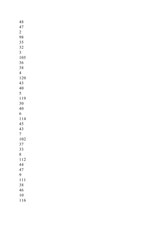
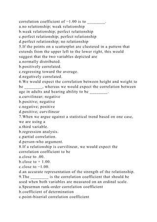
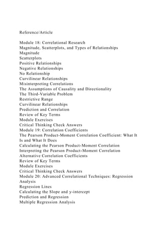
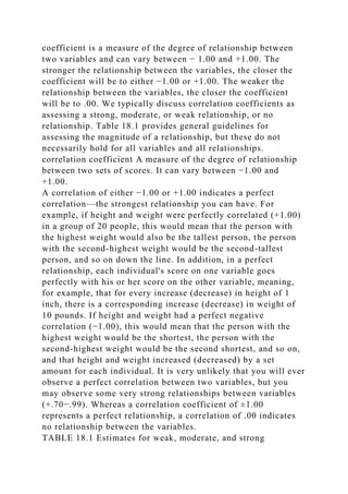
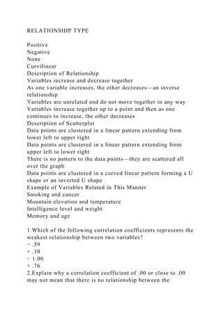
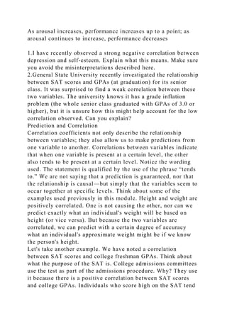
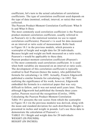
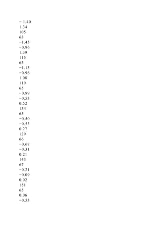
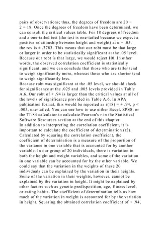
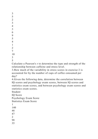
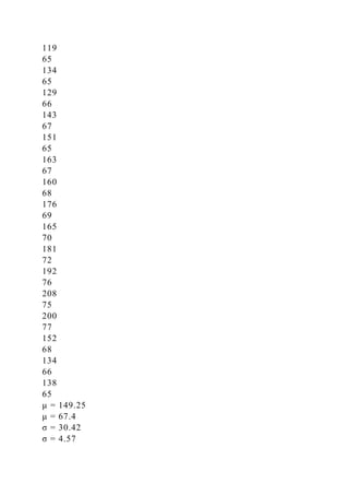
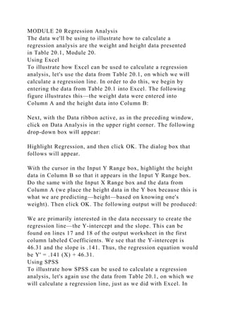
48. Next, click on Analyze, followed by Correlate, and
then Bivariate. The dialog box that follows will be produced.
Move the two variables you want correlated (Weight and
Height) into the Variables box. In addition, click One-
tailed because this was a one-tailed test, and lastly, click
on Options and select Means and standard deviations, thus
letting SPSS know that you want descriptive statistics on the
two variables. The dialog box should now appear as follows:
Click OK to receive the following output:
The correlation coefficient of +.941 is provided along with the
one-tailed significance level and the mean and standard
deviation for each of the variables.
Using the TI-84
Let's use the data from Table 19.1 to conduct the analysis using
the TI-84 calculator.
1.With the calculator on, press the STAT key.
2.EDIT will be highlighted. Press the ENTER key.
3.Under L1 enter the weight data from Table 19.1.
4.Under L2 enter the height data from Table 19.1.
5.Press the 2nd key and 0 [catalog] and scroll down to
DiagnosticOn and press ENTER. Press ENTER once again. (The
message DONE should appear on the screen.)
6.Press the STAT key and highlight CALC. Scroll down to
8:LinReg(a+ bx) and press ENTER.
7.Type L1 (by pressing the 2nd key followed by the 1 key)
followed by a comma and L2 (by pressing the 2nd key followed
by the 2 key) next to LinReg(a+ bx). It should appear as follows
on the screen: LinReg(a+ bx) L1,L2.
8.Press ENTER.
The values of a (46.31), b (.141), r2 (.89), and r (.94) should
appear on the screen. You can see that r (the correlation
coefficient) is the same as that calculated by Excel and SPSS.

49. MODULE 20 Regression Analysis
The data we'll be using to illustrate how to calculate a
regression analysis are the weight and height data presented
in Table 20.1, Module 20.
Using Excel
To illustrate how Excel can be used to calculate a regression
analysis, let's use the data from Table 20.1, on which we will
calculate a regression line. In order to do this, we begin by
entering the data from Table 20.1 into Excel. The following
figure illustrates this—the weight data were entered into
Column A and the height data into Column B:
Next, with the Data ribbon active, as in the preceding window,
click on Data Analysis in the upper right corner. The following
drop-down box will appear:
Highlight Regression, and then click OK. The dialog box that
follows will appear.
With the cursor in the Input Y Range box, highlight the height
data in Column B so that it appears in the Input Y Range box.
Do the same with the Input X Range box and the data from
Column A (we place the height data in the Y box because this is
what we are predicting—height—based on knowing one's
weight). Then click OK. The following output will be produced:
We are primarily interested in the data necessary to create the
regression line—the Y-intercept and the slope. This can be
found on lines 17 and 18 of the output worksheet in the first
column labeled Coefficients. We see that the Y-intercept is
46.31 and the slope is .141. Thus, the regression equation would
be Y' = .141 (X) + 46.31.
Using SPSS
To illustrate how SPSS can be used to calculate a regression
analysis, let's again use the data from Table 20.1, on which we
will calculate a regression line, just as we did with Excel. In

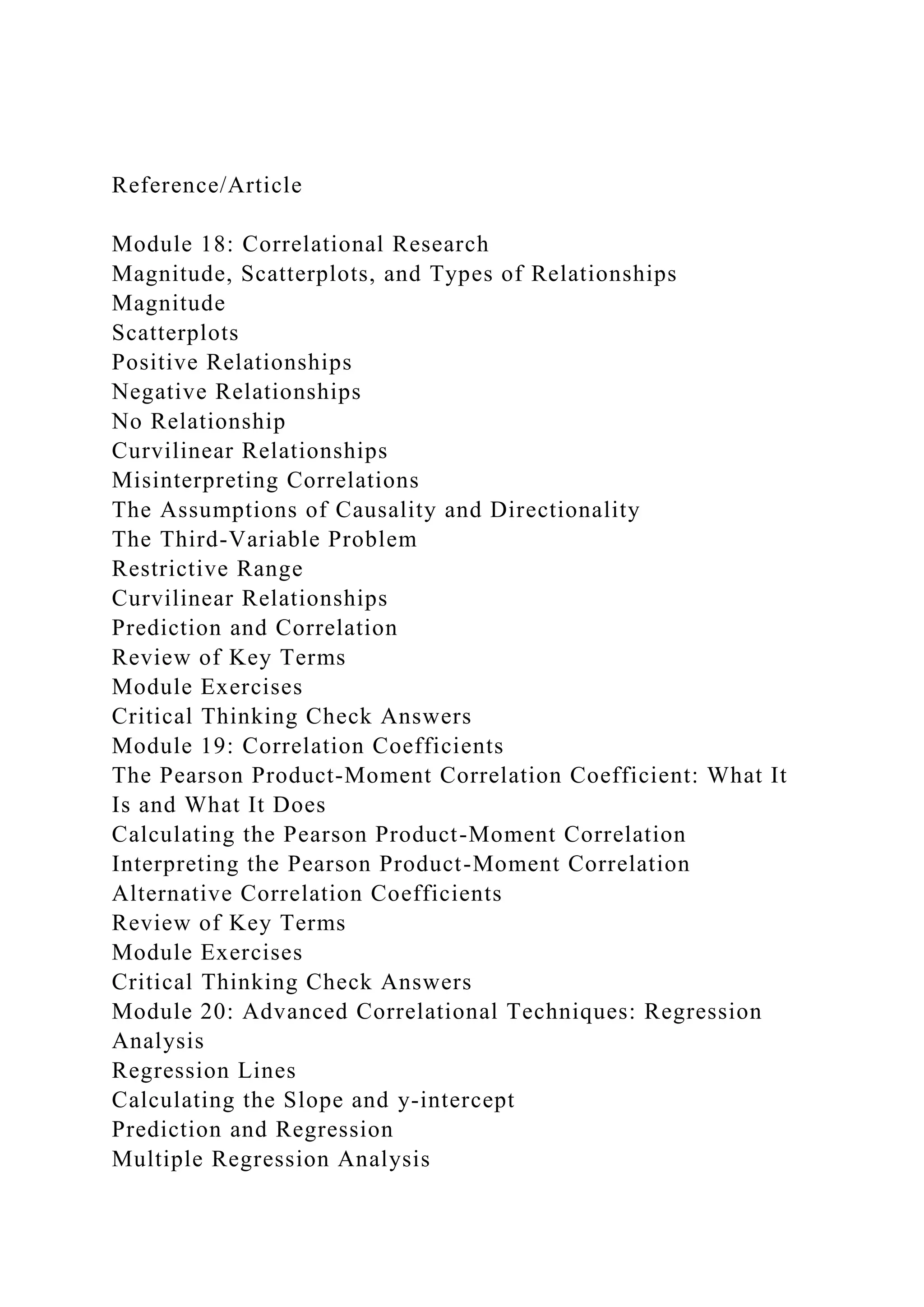
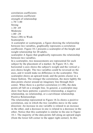
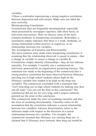
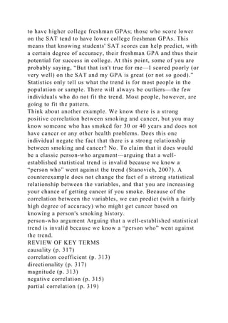
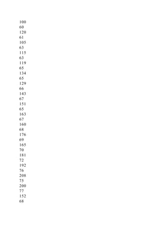
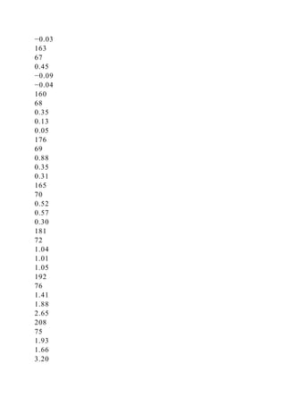
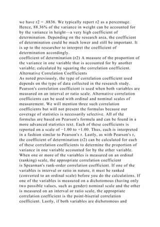
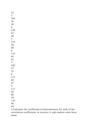
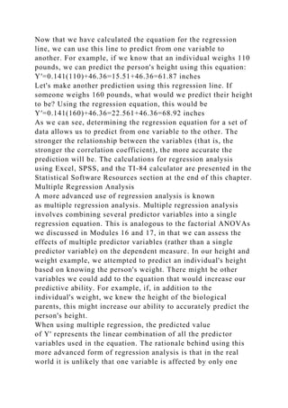
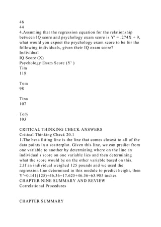
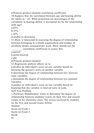
50. order to do this, we begin by entering the data from Table
20.1 into SPSS. The following figure illustrates this—the data
were entered just as they were when we used SPSS to calculate
a correlation coefficient in Module 20.
Next, click on Analyze, followed by Regression, and
then Linear, as in the following window:
The dialog box that follows will be produced.
For this regression analysis, we are attempting to predict height
based on knowing an individual's weight. Thus, we are using
height as the dependent measure in our model and weight as the
independent measure. Enter Height into the Dependent box and
Weight into the Independent box by using the appropriate
arrows. Then click OK. The output will be generated in the
output window.
We are most interested in the data necessary to create the
regression line—the Y-intercept and the slope. This can be
found in the box labeled Unstandardized Coefficients. We see
that the Y-intercept (Constant) is 46.314 and the slope is .141.
Thus, the regression equation would be Y' = .141 (X) + 46.31.
Using the TI-84
Let's use the data from Table 20.1 to conduct the regression
analysis using the TI-84 calculator.
1.With the calculator on, press the STAT key.
2.EDIT will be highlighted. Press the ENTER key.
3.Under L1 enter the weight data from Table 20.1.
4.Under L2 enter the height data from Table 20.1.
5.Press the 2nd key and 0 [catalog] and scroll down to
DiagnosticOn and press ENTER. Press ENTER once again. (The
message DONE should appear on the screen.)
6.Press the STAT key and highlight CALC. Scroll down to
8:LinReg(a + bx) and press ENTER.
7.Type L1 (by pressing the 2nd key followed by the 1 key)

51. followed by a comma and L2 (by pressing the 2nd key followed
by the 2 key) next to LinReg(a + bx). It should appear as
follows on the screen: LinReg(a + bx) L1,L2
8.Press ENTER.
The values of a (46.31), b (.141), r2 (.89), and r (.94) should
appear on the screen.
Assessment for and Challenges Related to Pervasive Mental
Illness and Health Concerns
In the 1950s, a radical shift in counseling occurred. Numerous
key figures in the fields of family counseling and therapy
proposed the view that pervasive mental health problems were
not individual problems, as was previously thought, but
originated with and were perpetuated by family dynamics. The
shift from working with individuals with pervasive or severe
mental illness or health concern via individual psychotherapy to
working with the identified “patient” and their families in the
1950s provided the context for the birth and growth of family
counseling/therapy. Since that time, mental health professionals
working with families with a member experiencing pervasive
mental illness or a health concern have moved away from the
controversial stance above, to acknowledge that both genes and
biology influence behavior and that relationships can maintain
or exacerbate symptomology as well as assist in alleviating it
via various coping mechanisms.
Tertiary intervention is the formal term for working with clients
experiencing pervasive mental illness or health concerns, but it
may also be referred to as remedial or rehabilitative counseling.
When you encounter a couple or family for which tertiary
intervention may be appropriate, your assessment focus should
shift. First, you should be cognizant of any symptoms or cues
that may substantiate your concerns, and if validated, you will
need to assess whether couple and family counseling is indeed

52. the best form of counseling service to provide. It may be that
one or more persons would benefit from individual services,
whether in conjunction with or as a precursor to any couple or
family counseling.
With these thoughts in mind:
DISSCUSSION a brief description of three symptoms/cues
observed in a family/couple session that may require assessment
and intervention beyond the scope of a family/couple session
and explain why. Then, explain how you, as a counselor, might
take the next steps with the individual who requires additional
assessment and intervention. Finally, explain any challenges of
continuing couple/family counseling once an individual requires
concurrent treatment.
Discussion: Please elaborate, discuss and give examples on the
3 questions below.
1.Why is the correlational method a predictive method? In other
words, how does establishing that two variables are correlated
allow us to make predictions? 275 words
2.Review this week’s course materials and learning activities,
and reflect on your learning so far this week. Respond to one or
more of the following prompts in one to two paragraphs: 275
words
a) Provide citation and reference to the material(s) you discuss.
Describe what you found interesting regarding this topic, and
why.
b) Describe how you will apply that learning in your daily life,
including your work life.
c) Describe what may be unclear to you, and what you would
like to learn.
3.Consider the following output for a Pearson's correlation:

53. Explain the table below, include the questions (a, b and c) 275
words
a) What does the negative sign tell you?
b) What does the significance level tell you?
c) How would you interpret this correlation in plain language?
Explain these answers thoroughly, as if you are explaining them
to someone who does not understand statistics. Correlation is
significant at the 0.05 level 92-tailed.
Explain these answers thoroughly, as if you are explaining them
to someone who does not understand statistics.
VAR00001
VAR00002
VAR00001 Pearson Correlation
Sig. (2-tailed)
N
1
8
-.800*
.017
8
VAR00002 Pearson Correlation
Sig. (2-tailed)
N
-.800*
.017
8
1
8