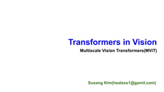
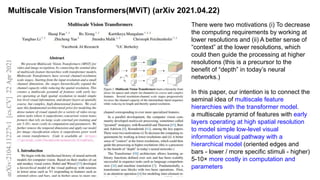
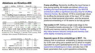
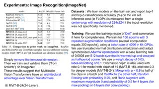
Susang Kim(healess1@gamil.com)
Transformers in Vision
Multiscale Vision Transformers(MViT)
Related work & References
Why Self-Attention
One is the total computational complexity per layer.
Another is the amount of computation that can be
parallelized, as measured by the minimum number
of sequential operations required. The third is the
path length between long-range dependencies in
the network.
Learning long-range dependencies is a key
challenge in many sequence transduction tasks. As
side benefit, self-attention could yield more
interpretable models. We inspect attention
distributions from our models.
Attention(Q,K,V) : Self-Attention Generative Adversarial Networks
Attention Is All You Need
self-attention models for
image recognition, object
detection, semantic and
instance segmentation, video
analysis and classification,
visual question answering,
visual commonsense
reasoning, image captioning,
vision language navigation,
clustering, few-shot learning,
and 3D data analysis.
Attention Is All You Need (NIPS 2017)
This lead to having more stable gradients
Transformer, the first sequence transduction model based entirely on attention, replacing the recurrent layers.
On Layer Normalization in the Transformer Architecture(ICML 2020)
Learning Deep Transformer Models for Machine Translation https://arxiv.org/pdf/1906.01787.pdf
In this paper, we study why the learning rate
warm-up stage is important in training the
Transformer and show that the location of
layer normalization matters.
Vision Transformer (ViT) (ICLR 2021)
An Image is Worth 16x16 Words: Transformers for Image Recognition at Scale
CNNs is not necessary and a pure transformer applied directly to sequences of image patches
Vision Transformer has much less image-specific inductive bias than CNNs
The sequence of linear embeddings of these patches
as an input to a Transformer. The Transformer encoder
consists of alternating layers of multi headed self
attention (MSA) and MLP blocks. Layernorm (LN) is
applied before every block, and residual connections
after every block
The Vision Transformer performs well when pre-trained on a large
JFT-300M dataset. With fewer inductive biases for vision than ResNets.
※ JFT-300M Dataset (300M web images / ~ 19K categories)
Is Space-Time Attention All You Need for Video Understanding? (ICML 2021)
“TimeSformer,” adapts the standard Transformer architecture to video by enabling spatiotemporal feature learning
directly from a sequence of framelevel patches.
Sequence of frame-level patches with a size of 16 × 16
pixels. query patch and show in non-blue colors its
self-attention space-time neighborhood under each scheme.
Patches without color are not used for the self-attention
computation of the blue patch. Multiple colors within a
scheme denote attentions separately applied along different
dimensions (e.g., space and time for (T+S)) or over different
neighborhoods (e.g., for (L+G)). Note that self-attention is
computed for every single patch in the video clip, every
patch serves as a query. it extends in the same fashion to
all frames of the clip
DeiT (Data-efficient image Transformers) (ICML 2021)
Training data-efficient image transformers & distillation through attention
In this paper, we have introduced DeiT, which are image transformers that do not require
very large amount of data to be trained. we train a vision transformer on a single 8-GPU
node in two to three days (53 hours of pre-training, and optionally 20 hours of fine-tuning)
that is competitive with convnets having a similar number of parameters and efficiency.
ViViT: A Video Vision Transformer (arXiv 2021.03.29)
Pure-transformer based models for video classification, we propose several,
efficient variants of our model which factorise the spatial- and temporal-dimensions
of the input. how we can effectively regularise the model during training and
leverage pretrained image models to be able to train on comparatively small
datasets.
Model 1: Spatio-temporal attention : all spatio-temporal tokens
Model 2: Factorised encoder : two separate transformer encoders
Model 3: Factorised self-attention : the order of spatial-then-temporal selfattention
Model 4: Factorised dot-product attention :
Multiscale Vision Transformers(MViT)
Multiscale Vision Transformers(MViT) (arXiv 2021.04.22)
There were two motivations (i) To decrease
the computing requirements by working at
lower resolutions and (ii) A better sense of
“context” at the lower resolutions, which
could then guide the processing at higher
resolutions (this is a precursor to the
benefit of “depth” in today’s neural
networks.)
In this paper, our intention is to connect the
seminal idea of multiscale feature
hierarchies with the transformer model.
a multiscale pyramid of features with early
layers operating at high spatial resolution
to model simple low-level visual
information visual pathway with a
hierarchical model (oriented edges and
bars - lower / more specific stimuli - higher)
5-10× more costly in computation and
parameters
Transformer architecture MViT builds on the core concept of stages. Each
stage consists of multiple transformer blocks with
specific space-time resolution and channel
dimension. The main idea of Multiscale
Transformers is to progressively expand the
channel capacity, while pooling the resolution from
input to output of the network
Multiscale Transformers have several
channel-resolution ‘scale’ stages. Starting from the
image resolution and a small channel dimension,
the stages hierarchically expand the channel
capacity while reducing the spatial resolution
This creates a multiscale pyramid of feature
activations inside the transformer network,
effectively connecting the principles of
transformers with multi scale feature hierarchies.
The early layers of our architecture can operate at high spatial resolution to model simple low-level visual
information, due to the lightweight channel capacity. In turn, the deeper layers can effectively focus on
spatially coarse but complex high-level features to model visual semantics. The fundamental advantage
of our multiscale transformer arises from the extremely dense nature of visual signals, a phenomenon
that is even more pronounced for space-time visual signals captured in video.
Multi Head Pooling Attention(MHPA)
Multiscale Transformers to operate at progressively changing spatio-temporal resolution.(a self attention
operator that enables flexible resolution modeling in a transformer block allowing)
Multi Head Attention (MHA) operators,
where the channel dimension
and the spatiotemporal resolution remains fixed,
MHPA pools the sequence of latent tensors
to reduce the sequence length
(resolution) of the attended input.
Multi Head Pooling Attention(MHPA)
Pooling Operator. The operator P(·; Θ) performs a pooling kernel computation on the input tensor along
each of the dimensions. Unpacking Θ as Θ := (k, s, p) (kernel, stride, padding) input tensor of dimensions L
= T × H × W to L˜ given by,
Pooling Attention. The pooling operator P(·; Θ) is applied to all the intermediate tensors Qˆ, Kˆ and Vˆ
independently with chosen pooling kernels k, stride s and padding p. Denoting θ yielding the pre-attention
vectors Q = P(Qˆ; ΘQ), K = P(Kˆ ; ΘK) and V = P(Vˆ ; ΘV ) with reduced sequence lengths. Attention is now
computed on these shortened vectors, with the operation,
Multiple heads. computation can be parallelized by considering h heads where each head is performing
the pooling attention on a non overlapping subset of D/h channels of the D dimensional input tensor X.
Computational Analysis. the sequence length, pooling the key, query and value tensors has dramatic
benefits on the fundamental compute and memory requirements of the Multiscale Transformer model.
ViT vs MViT
MViT architecture has fine spacetime (and coarse
channel) resolution in early layers that is
up-/downsampled to a coarse spacetime (and fine
channel) resolution in late layers.
ViT maintains a constant channel capacity and spatial
resolution throughout all the blocks.This is equivalent
to a convolution with equal kernel size and stride of
1×16×16 and is shown as patch1 stage in the model
definition in Table 1. sequence of length L with
dimension D to encode the positional information and
break permutation invariance.
Multiscale Transformer Networks
1.Scale stages : the channel dimension of the processed sequence is upsampled while the length of the sequence is
down-sampled. This effectively reduces the spatio-temporal resolution of the underlying visual data while allowing the
network to assimilate the processed information in more complex features.
2.Channel expansion : we expand the channel dimension by increasing the output of the final MLP layer in the previous
stage by a factor that is relative to the resolution change introduced at the stage. down-sample the space-time resolution by
4×, we increase the channel dimension by 2×.
3.Query pooling : The pooling attention operation affords flexibility not only in the length of key and value vectors but also in
the length of the query, and thereby output, sequence. our intention is to decrease resolution at the beginning of a stage and
then preserve this resolution throughout the stage
4.Key-Value pooling : We decouple the usage of K, V and Q pooling, with Q pooling being used in the first layer of each
stage and K, V pooling being employed in all other layers. Since the sequence length of key and value tensors need to be
identical to allow attention weight calculation, the pooling stride used on K and value V tensors needs to be identical. In our
default setting, we constrain all pooling parameters (k; p; s) to be identical i.e. ΘK ≡ ΘV within a stage, but vary s adaptively
w.r.t. to the scale across stages.
5.Skip connections : MHPA handles this mismatch by adding the query pooling operator P(·; ΘQ) to the residual path.
instead of directly adding the input X of MHPA to the output, we add the pooled input X to the output, thereby matching the
resolution to attended query Q. For handling the channel dimension mismatch between stage changes, we employ an extra
linear layer that operates on the layer-normalized output of our MHPA operation. Note that this differs from the other
(resolution-preserving) skip connections that operate on the un-normalized signal.
Network instantiation details
ViT-Base input to patches of shape 1×16×16 with dimension D = 768, followed by stacking N = 12 transformer blocks. With an
8×224×224 input the resolution is fixed to 768×8×14×14 throughout all layers. The sequence length (spacetime resolution + class
token) is 8 · 14 · 14 + 1(classification task) = 1569.
MViT-B input to a channel dimension of D = 96 with overlapping space-time cubes of shape 3×7×7. The resulting sequence of
length 8 ∗ 56 ∗ 56 + 1 = 25089 is reduced by a factor of 4 for each additional stage, to a final sequence length of 8 ∗ 7 ∗ 7 + 1 =
393 at scale4. In tandem, the channel dimension is up-sampled by a factor of 2 at each stage, increasing to 768 at scale4. Note
that all pooling operations, and hence the resolution downsampling, We set the number of MHPA heads to h = 1 in the scale1
stage and increase the number of heads with the channel dimension (channels per-head D/h remain consistent at 96). At each
stage transition, the previous stage output MLP dimension is increased by 2× and MHPA pools on Q tensors.
Experiments: Video Recognition(Kinetics-400)
Datasets. Kinetics-400 (∼240k training videos in 400 classes) report
top-1 and top-5 classification accuracy (%) on the validation set,
computational cost (in FLOPs) of a single, spatially center-cropped
clip and the number of clips used.
Training. random initialization (“from scratch”) on Kinetics, without
using ImageNet or other pre-training. For Kinetics, we train for 200
epochs with 2 repeated augmentation repetitions. We report ViT
baselines that are fine-tuned from ImageNet, using a 30-epoch
version of the training recipe in SlowFast. For the temporal domain,
we sample a clip from the full length video, and the input to the
network are T frames with a temporal stride of τ ; denoted as T × τ.
Inference. We apply two testing strategies following: (i) Temporally,
uniformly samples K clips (e.g. K=5) from a video, scales the shorter
spatial side to 256 pixels and takes a 224×224 center crop, and (ii),
the same as (i) temporally, but take 3 crops of 224×224 to cover the
longer spatial axis. We average the scores for all individual
predictions.
Optimization details. adopt synchronized AdamW training on 128
GPUs. we train for 200 epochs with 2 repeated augmentation
repetitions. The mini-batch size is 4 clips per GPU (so the overall
batchsize is 512). use a linear warm-up strategy in the first 30
epochs.
Ablations on Kinetics-400
Frame shuffling. Randomly shuffling the input frames in
time during testing. All models are trained without any
shuffling and have temporal embeddings. Our MViT-B
architecture suffers a significant accuracy drop for shuffling
inference frames. By contrast, ViT-B is surprisingly robust
for shuffling the temporal order of the input. ViT to video
does not model temporal information, and the temporal
positional embedding in ViT-B seems to be fully ignored.
Two scales in ViT. Adding a single scale stage to the
ViT-B baseline boosts accuracy by +1.5% while deceasing
FLOPs and memory cost by 38% and 41%. Pooling
Key-Value tensors reduces compute and memory cost
while slightly increasing accuracy.
Separate space & time embeddings in MViT. We
observe that no positional embedding (i) decays accuracy
by -0.9% over using just a spatial one (ii) which is roughly
equivalent to a joint spatiotemporal one (iii). Our separate
space-time embedding (iv) is best, and also has 2.1M
fewer parameters than a joint spacetime embedding.
Ablations on Kinetics-400
Input Sampling Rate. different cubification kernel size c and
sampling stride s. sampling patches, cT = 1, performs worse than
sampling cubes with cT > 1. Also, sampling overlapping input
cubes s < c allows better information flow and benefits
performance. While cT > 1 helps, very large temporal kernel size
(cT = 7) doesn’t futher improve performance.
Stage distribution. The overall number of transformer blocks,
N=16 is consistent. We observe that having more blocks in early
stages increases memory and having more blocks later stages the
parameters of the architecture. Shifting the majority of blocks to the
scale4 stage achieves the best trade-off.
Speed-Accuracy tradeoff. We measure training throughput as the
number of video clips per second on a single M40 GPU. MViT-S
and MViT-B models are not only significantly more accurate but
also much faster than both the ViT-B baseline and convolutional
models. Using a conv instead of maxpooling in MHSA, we observe
a training speed reduction of ∼20% for convolution and additional
parameter updates.
Experiments: Image Recognition(ImageNet)
Simply remove the temporal dimension.
Then we train and validate them (“from
scratch”) on ImageNet
These results suggest that Multiscale
Vision Transformers have an architectural
advantage over Vision Transformers.
※ MViT-B-24(24-Layer)
Datasets : We train models on the train set and report top-1
and top-5 classification accuracy (%) on the val set.
Inference cost (in FLOPs) is measured from a single
center-crop with resolution of 224x224 if the input resolution
was not specifically mentioned.
Training. We use the training recipe of DeiT and summarize
it here for completeness. We train for 100 epochs with 3
repeated augmentation repetitions (overall computation
equals 300 epochs), using a batch size of 4096 in 64 GPUs.
We use truncated normal distribution initialization and adopt
synchronized AdamW optimization with a base learning rate
of 0.0005 per 512 batch-size that is warmed up and decayed
as half-period cosine. We use a weight decay of 0.05,
label-smoothing of 0.1. Stochastic depth is also used with
rate 0.1 for model with depth of 16 (MViT-B-16), and rate 0.3
for deeper models (MViT-B-24). Mixup with α = 0.8 to half of
the clips in a batch and CutMix to the other half, Random
Erasing with probability 0.25, and Rand Augment with
maximum magnitude 9 and probability of 0.5 for 4 layers (for
max-pooling) or 6 layers (for conv-pooling).
Accuracy/complexity trade-off
More importantly, the MViT result is achieved without external data.
All concurrent Transformer based works require the huge scale ImageNet-21K to be competitive, and
the performance degrades significantly. These works further report failure of training without ImageNet
initialization. MViT-B compute/accuracy trade-off is similar to X3D-XL.
Codes
# MViT options (/slowfast/config/defaults.py)
_C.MVIT = CfgNode()
_C.MVIT.PATCH_KERNEL = [3, 7, 7]  _C.MVIT.PATCH_STRIDE = [2, 4, 4]  _C.MVIT.PATCH_PADDING = [2, 4, 4]
_C.MVIT.EMBED_DIM = 96  _C.MVIT.MLP_RATIO = 4.0  _C.MVIT.DEPTH = 16  _C.MVIT.NORM = "layernorm"
# MViT options (/slowfast/models/video_model_builder.py)
@MODEL_REGISTRY.register()
class MViT(nn.Module):
if cfg.MVIT.NORM == "layernorm":
norm_layer = partial(nn.LayerNorm, eps=1e-6)
self.patch_dims = [
self.input_dims[i] // self.patch_stride[i]
for i in range(len(self.input_dims))
]
num_patches = math.prod(self.patch_dims)
dim_mul, head_mul = torch.ones(depth + 1), torch.ones(depth + 1)
for i in range(len(cfg.MVIT.DIM_MUL)):
dim_mul[cfg.MVIT.DIM_MUL[i][0]] = cfg.MVIT.DIM_MUL[i][1]
for i in range(len(cfg.MVIT.HEAD_MUL)):
head_mul[cfg.MVIT.HEAD_MUL[i][0]] = cfg.MVIT.HEAD_MUL[i][1]
https://github1s.com/facebookresearch/SlowFast/blob/master/slowfast/config/defaults.py
Codes
for i in range(len(cfg.MVIT.POOL_Q_STRIDE)):
for i in range(len(cfg.MVIT.POOL_KV_STRIDE)):
for i in range(depth):
num_heads = round_width(num_heads, head_mul[i])
embed_dim = round_width(embed_dim, dim_mul[i], divisor=num_heads)
dim_out = round_width( embed_dim, dim_mul[i + 1],
divisor=round_width(num_heads, head_mul[i + 1]),
)
self.blocks.append(
MultiScaleBlock(
dim=embed_dim, dim_out=dim_out, num_heads=num_heads, mlp_ratio=mlp_ratio,
qkv_bias=qkv_bias, drop_rate=self.drop_rate, drop_path=dpr[i], norm_layer=norm_layer,
kernel_q=pool_q[i] if len(pool_q) > i else [],
kernel_kv=pool_kv[i] if len(pool_kv) > i else [],
stride_q=stride_q[i] if len(stride_q) > i else [],
stride_kv=stride_kv[i] if len(stride_kv) > i else [],
mode=mode, has_cls_embed=self.cls_embed_on, pool_first=pool_first,
)
)
https://github1s.com/facebookresearch/SlowFast/blob/master/slowfast/models/video_model_builder.py
Thanks
Any Questions?
You can send mail to
Susang Kim(healess1@gmail.com)

[Paper] Multiscale Vision Transformers(MVit)

  • 1.
    Susang Kim(healess1@gamil.com) Transformers inVision Multiscale Vision Transformers(MViT)
  • 2.
    Related work &References
  • 3.
    Why Self-Attention One isthe total computational complexity per layer. Another is the amount of computation that can be parallelized, as measured by the minimum number of sequential operations required. The third is the path length between long-range dependencies in the network. Learning long-range dependencies is a key challenge in many sequence transduction tasks. As side benefit, self-attention could yield more interpretable models. We inspect attention distributions from our models. Attention(Q,K,V) : Self-Attention Generative Adversarial Networks Attention Is All You Need self-attention models for image recognition, object detection, semantic and instance segmentation, video analysis and classification, visual question answering, visual commonsense reasoning, image captioning, vision language navigation, clustering, few-shot learning, and 3D data analysis.
  • 4.
    Attention Is AllYou Need (NIPS 2017) This lead to having more stable gradients Transformer, the first sequence transduction model based entirely on attention, replacing the recurrent layers.
  • 5.
    On Layer Normalizationin the Transformer Architecture(ICML 2020) Learning Deep Transformer Models for Machine Translation https://arxiv.org/pdf/1906.01787.pdf In this paper, we study why the learning rate warm-up stage is important in training the Transformer and show that the location of layer normalization matters.
  • 6.
    Vision Transformer (ViT)(ICLR 2021) An Image is Worth 16x16 Words: Transformers for Image Recognition at Scale CNNs is not necessary and a pure transformer applied directly to sequences of image patches Vision Transformer has much less image-specific inductive bias than CNNs The sequence of linear embeddings of these patches as an input to a Transformer. The Transformer encoder consists of alternating layers of multi headed self attention (MSA) and MLP blocks. Layernorm (LN) is applied before every block, and residual connections after every block The Vision Transformer performs well when pre-trained on a large JFT-300M dataset. With fewer inductive biases for vision than ResNets. ※ JFT-300M Dataset (300M web images / ~ 19K categories)
  • 7.
    Is Space-Time AttentionAll You Need for Video Understanding? (ICML 2021) “TimeSformer,” adapts the standard Transformer architecture to video by enabling spatiotemporal feature learning directly from a sequence of framelevel patches. Sequence of frame-level patches with a size of 16 × 16 pixels. query patch and show in non-blue colors its self-attention space-time neighborhood under each scheme. Patches without color are not used for the self-attention computation of the blue patch. Multiple colors within a scheme denote attentions separately applied along different dimensions (e.g., space and time for (T+S)) or over different neighborhoods (e.g., for (L+G)). Note that self-attention is computed for every single patch in the video clip, every patch serves as a query. it extends in the same fashion to all frames of the clip
  • 8.
    DeiT (Data-efficient imageTransformers) (ICML 2021) Training data-efficient image transformers & distillation through attention In this paper, we have introduced DeiT, which are image transformers that do not require very large amount of data to be trained. we train a vision transformer on a single 8-GPU node in two to three days (53 hours of pre-training, and optionally 20 hours of fine-tuning) that is competitive with convnets having a similar number of parameters and efficiency.
  • 9.
    ViViT: A VideoVision Transformer (arXiv 2021.03.29) Pure-transformer based models for video classification, we propose several, efficient variants of our model which factorise the spatial- and temporal-dimensions of the input. how we can effectively regularise the model during training and leverage pretrained image models to be able to train on comparatively small datasets. Model 1: Spatio-temporal attention : all spatio-temporal tokens Model 2: Factorised encoder : two separate transformer encoders Model 3: Factorised self-attention : the order of spatial-then-temporal selfattention Model 4: Factorised dot-product attention :
  • 10.
  • 11.
    Multiscale Vision Transformers(MViT)(arXiv 2021.04.22) There were two motivations (i) To decrease the computing requirements by working at lower resolutions and (ii) A better sense of “context” at the lower resolutions, which could then guide the processing at higher resolutions (this is a precursor to the benefit of “depth” in today’s neural networks.) In this paper, our intention is to connect the seminal idea of multiscale feature hierarchies with the transformer model. a multiscale pyramid of features with early layers operating at high spatial resolution to model simple low-level visual information visual pathway with a hierarchical model (oriented edges and bars - lower / more specific stimuli - higher) 5-10× more costly in computation and parameters
  • 12.
    Transformer architecture MViTbuilds on the core concept of stages. Each stage consists of multiple transformer blocks with specific space-time resolution and channel dimension. The main idea of Multiscale Transformers is to progressively expand the channel capacity, while pooling the resolution from input to output of the network Multiscale Transformers have several channel-resolution ‘scale’ stages. Starting from the image resolution and a small channel dimension, the stages hierarchically expand the channel capacity while reducing the spatial resolution This creates a multiscale pyramid of feature activations inside the transformer network, effectively connecting the principles of transformers with multi scale feature hierarchies. The early layers of our architecture can operate at high spatial resolution to model simple low-level visual information, due to the lightweight channel capacity. In turn, the deeper layers can effectively focus on spatially coarse but complex high-level features to model visual semantics. The fundamental advantage of our multiscale transformer arises from the extremely dense nature of visual signals, a phenomenon that is even more pronounced for space-time visual signals captured in video.
  • 13.
    Multi Head PoolingAttention(MHPA) Multiscale Transformers to operate at progressively changing spatio-temporal resolution.(a self attention operator that enables flexible resolution modeling in a transformer block allowing) Multi Head Attention (MHA) operators, where the channel dimension and the spatiotemporal resolution remains fixed, MHPA pools the sequence of latent tensors to reduce the sequence length (resolution) of the attended input.
  • 14.
    Multi Head PoolingAttention(MHPA) Pooling Operator. The operator P(·; Θ) performs a pooling kernel computation on the input tensor along each of the dimensions. Unpacking Θ as Θ := (k, s, p) (kernel, stride, padding) input tensor of dimensions L = T × H × W to L˜ given by, Pooling Attention. The pooling operator P(·; Θ) is applied to all the intermediate tensors Qˆ, Kˆ and Vˆ independently with chosen pooling kernels k, stride s and padding p. Denoting θ yielding the pre-attention vectors Q = P(Qˆ; ΘQ), K = P(Kˆ ; ΘK) and V = P(Vˆ ; ΘV ) with reduced sequence lengths. Attention is now computed on these shortened vectors, with the operation, Multiple heads. computation can be parallelized by considering h heads where each head is performing the pooling attention on a non overlapping subset of D/h channels of the D dimensional input tensor X. Computational Analysis. the sequence length, pooling the key, query and value tensors has dramatic benefits on the fundamental compute and memory requirements of the Multiscale Transformer model.
  • 15.
    ViT vs MViT MViTarchitecture has fine spacetime (and coarse channel) resolution in early layers that is up-/downsampled to a coarse spacetime (and fine channel) resolution in late layers. ViT maintains a constant channel capacity and spatial resolution throughout all the blocks.This is equivalent to a convolution with equal kernel size and stride of 1×16×16 and is shown as patch1 stage in the model definition in Table 1. sequence of length L with dimension D to encode the positional information and break permutation invariance.
  • 16.
    Multiscale Transformer Networks 1.Scalestages : the channel dimension of the processed sequence is upsampled while the length of the sequence is down-sampled. This effectively reduces the spatio-temporal resolution of the underlying visual data while allowing the network to assimilate the processed information in more complex features. 2.Channel expansion : we expand the channel dimension by increasing the output of the final MLP layer in the previous stage by a factor that is relative to the resolution change introduced at the stage. down-sample the space-time resolution by 4×, we increase the channel dimension by 2×. 3.Query pooling : The pooling attention operation affords flexibility not only in the length of key and value vectors but also in the length of the query, and thereby output, sequence. our intention is to decrease resolution at the beginning of a stage and then preserve this resolution throughout the stage 4.Key-Value pooling : We decouple the usage of K, V and Q pooling, with Q pooling being used in the first layer of each stage and K, V pooling being employed in all other layers. Since the sequence length of key and value tensors need to be identical to allow attention weight calculation, the pooling stride used on K and value V tensors needs to be identical. In our default setting, we constrain all pooling parameters (k; p; s) to be identical i.e. ΘK ≡ ΘV within a stage, but vary s adaptively w.r.t. to the scale across stages. 5.Skip connections : MHPA handles this mismatch by adding the query pooling operator P(·; ΘQ) to the residual path. instead of directly adding the input X of MHPA to the output, we add the pooled input X to the output, thereby matching the resolution to attended query Q. For handling the channel dimension mismatch between stage changes, we employ an extra linear layer that operates on the layer-normalized output of our MHPA operation. Note that this differs from the other (resolution-preserving) skip connections that operate on the un-normalized signal.
  • 17.
    Network instantiation details ViT-Baseinput to patches of shape 1×16×16 with dimension D = 768, followed by stacking N = 12 transformer blocks. With an 8×224×224 input the resolution is fixed to 768×8×14×14 throughout all layers. The sequence length (spacetime resolution + class token) is 8 · 14 · 14 + 1(classification task) = 1569. MViT-B input to a channel dimension of D = 96 with overlapping space-time cubes of shape 3×7×7. The resulting sequence of length 8 ∗ 56 ∗ 56 + 1 = 25089 is reduced by a factor of 4 for each additional stage, to a final sequence length of 8 ∗ 7 ∗ 7 + 1 = 393 at scale4. In tandem, the channel dimension is up-sampled by a factor of 2 at each stage, increasing to 768 at scale4. Note that all pooling operations, and hence the resolution downsampling, We set the number of MHPA heads to h = 1 in the scale1 stage and increase the number of heads with the channel dimension (channels per-head D/h remain consistent at 96). At each stage transition, the previous stage output MLP dimension is increased by 2× and MHPA pools on Q tensors.
  • 18.
    Experiments: Video Recognition(Kinetics-400) Datasets.Kinetics-400 (∼240k training videos in 400 classes) report top-1 and top-5 classification accuracy (%) on the validation set, computational cost (in FLOPs) of a single, spatially center-cropped clip and the number of clips used. Training. random initialization (“from scratch”) on Kinetics, without using ImageNet or other pre-training. For Kinetics, we train for 200 epochs with 2 repeated augmentation repetitions. We report ViT baselines that are fine-tuned from ImageNet, using a 30-epoch version of the training recipe in SlowFast. For the temporal domain, we sample a clip from the full length video, and the input to the network are T frames with a temporal stride of τ ; denoted as T × τ. Inference. We apply two testing strategies following: (i) Temporally, uniformly samples K clips (e.g. K=5) from a video, scales the shorter spatial side to 256 pixels and takes a 224×224 center crop, and (ii), the same as (i) temporally, but take 3 crops of 224×224 to cover the longer spatial axis. We average the scores for all individual predictions. Optimization details. adopt synchronized AdamW training on 128 GPUs. we train for 200 epochs with 2 repeated augmentation repetitions. The mini-batch size is 4 clips per GPU (so the overall batchsize is 512). use a linear warm-up strategy in the first 30 epochs.
  • 19.
    Ablations on Kinetics-400 Frameshuffling. Randomly shuffling the input frames in time during testing. All models are trained without any shuffling and have temporal embeddings. Our MViT-B architecture suffers a significant accuracy drop for shuffling inference frames. By contrast, ViT-B is surprisingly robust for shuffling the temporal order of the input. ViT to video does not model temporal information, and the temporal positional embedding in ViT-B seems to be fully ignored. Two scales in ViT. Adding a single scale stage to the ViT-B baseline boosts accuracy by +1.5% while deceasing FLOPs and memory cost by 38% and 41%. Pooling Key-Value tensors reduces compute and memory cost while slightly increasing accuracy. Separate space & time embeddings in MViT. We observe that no positional embedding (i) decays accuracy by -0.9% over using just a spatial one (ii) which is roughly equivalent to a joint spatiotemporal one (iii). Our separate space-time embedding (iv) is best, and also has 2.1M fewer parameters than a joint spacetime embedding.
  • 20.
    Ablations on Kinetics-400 InputSampling Rate. different cubification kernel size c and sampling stride s. sampling patches, cT = 1, performs worse than sampling cubes with cT > 1. Also, sampling overlapping input cubes s < c allows better information flow and benefits performance. While cT > 1 helps, very large temporal kernel size (cT = 7) doesn’t futher improve performance. Stage distribution. The overall number of transformer blocks, N=16 is consistent. We observe that having more blocks in early stages increases memory and having more blocks later stages the parameters of the architecture. Shifting the majority of blocks to the scale4 stage achieves the best trade-off. Speed-Accuracy tradeoff. We measure training throughput as the number of video clips per second on a single M40 GPU. MViT-S and MViT-B models are not only significantly more accurate but also much faster than both the ViT-B baseline and convolutional models. Using a conv instead of maxpooling in MHSA, we observe a training speed reduction of ∼20% for convolution and additional parameter updates.
  • 21.
    Experiments: Image Recognition(ImageNet) Simplyremove the temporal dimension. Then we train and validate them (“from scratch”) on ImageNet These results suggest that Multiscale Vision Transformers have an architectural advantage over Vision Transformers. ※ MViT-B-24(24-Layer) Datasets : We train models on the train set and report top-1 and top-5 classification accuracy (%) on the val set. Inference cost (in FLOPs) is measured from a single center-crop with resolution of 224x224 if the input resolution was not specifically mentioned. Training. We use the training recipe of DeiT and summarize it here for completeness. We train for 100 epochs with 3 repeated augmentation repetitions (overall computation equals 300 epochs), using a batch size of 4096 in 64 GPUs. We use truncated normal distribution initialization and adopt synchronized AdamW optimization with a base learning rate of 0.0005 per 512 batch-size that is warmed up and decayed as half-period cosine. We use a weight decay of 0.05, label-smoothing of 0.1. Stochastic depth is also used with rate 0.1 for model with depth of 16 (MViT-B-16), and rate 0.3 for deeper models (MViT-B-24). Mixup with α = 0.8 to half of the clips in a batch and CutMix to the other half, Random Erasing with probability 0.25, and Rand Augment with maximum magnitude 9 and probability of 0.5 for 4 layers (for max-pooling) or 6 layers (for conv-pooling).
  • 22.
    Accuracy/complexity trade-off More importantly,the MViT result is achieved without external data. All concurrent Transformer based works require the huge scale ImageNet-21K to be competitive, and the performance degrades significantly. These works further report failure of training without ImageNet initialization. MViT-B compute/accuracy trade-off is similar to X3D-XL.
  • 23.
    Codes # MViT options(/slowfast/config/defaults.py) _C.MVIT = CfgNode() _C.MVIT.PATCH_KERNEL = [3, 7, 7] _C.MVIT.PATCH_STRIDE = [2, 4, 4] _C.MVIT.PATCH_PADDING = [2, 4, 4] _C.MVIT.EMBED_DIM = 96 _C.MVIT.MLP_RATIO = 4.0 _C.MVIT.DEPTH = 16 _C.MVIT.NORM = "layernorm" # MViT options (/slowfast/models/video_model_builder.py) @MODEL_REGISTRY.register() class MViT(nn.Module): if cfg.MVIT.NORM == "layernorm": norm_layer = partial(nn.LayerNorm, eps=1e-6) self.patch_dims = [ self.input_dims[i] // self.patch_stride[i] for i in range(len(self.input_dims)) ] num_patches = math.prod(self.patch_dims) dim_mul, head_mul = torch.ones(depth + 1), torch.ones(depth + 1) for i in range(len(cfg.MVIT.DIM_MUL)): dim_mul[cfg.MVIT.DIM_MUL[i][0]] = cfg.MVIT.DIM_MUL[i][1] for i in range(len(cfg.MVIT.HEAD_MUL)): head_mul[cfg.MVIT.HEAD_MUL[i][0]] = cfg.MVIT.HEAD_MUL[i][1] https://github1s.com/facebookresearch/SlowFast/blob/master/slowfast/config/defaults.py
  • 24.
    Codes for i inrange(len(cfg.MVIT.POOL_Q_STRIDE)): for i in range(len(cfg.MVIT.POOL_KV_STRIDE)): for i in range(depth): num_heads = round_width(num_heads, head_mul[i]) embed_dim = round_width(embed_dim, dim_mul[i], divisor=num_heads) dim_out = round_width( embed_dim, dim_mul[i + 1], divisor=round_width(num_heads, head_mul[i + 1]), ) self.blocks.append( MultiScaleBlock( dim=embed_dim, dim_out=dim_out, num_heads=num_heads, mlp_ratio=mlp_ratio, qkv_bias=qkv_bias, drop_rate=self.drop_rate, drop_path=dpr[i], norm_layer=norm_layer, kernel_q=pool_q[i] if len(pool_q) > i else [], kernel_kv=pool_kv[i] if len(pool_kv) > i else [], stride_q=stride_q[i] if len(stride_q) > i else [], stride_kv=stride_kv[i] if len(stride_kv) > i else [], mode=mode, has_cls_embed=self.cls_embed_on, pool_first=pool_first, ) ) https://github1s.com/facebookresearch/SlowFast/blob/master/slowfast/models/video_model_builder.py
  • 25.
    Thanks Any Questions? You cansend mail to Susang Kim(healess1@gmail.com)