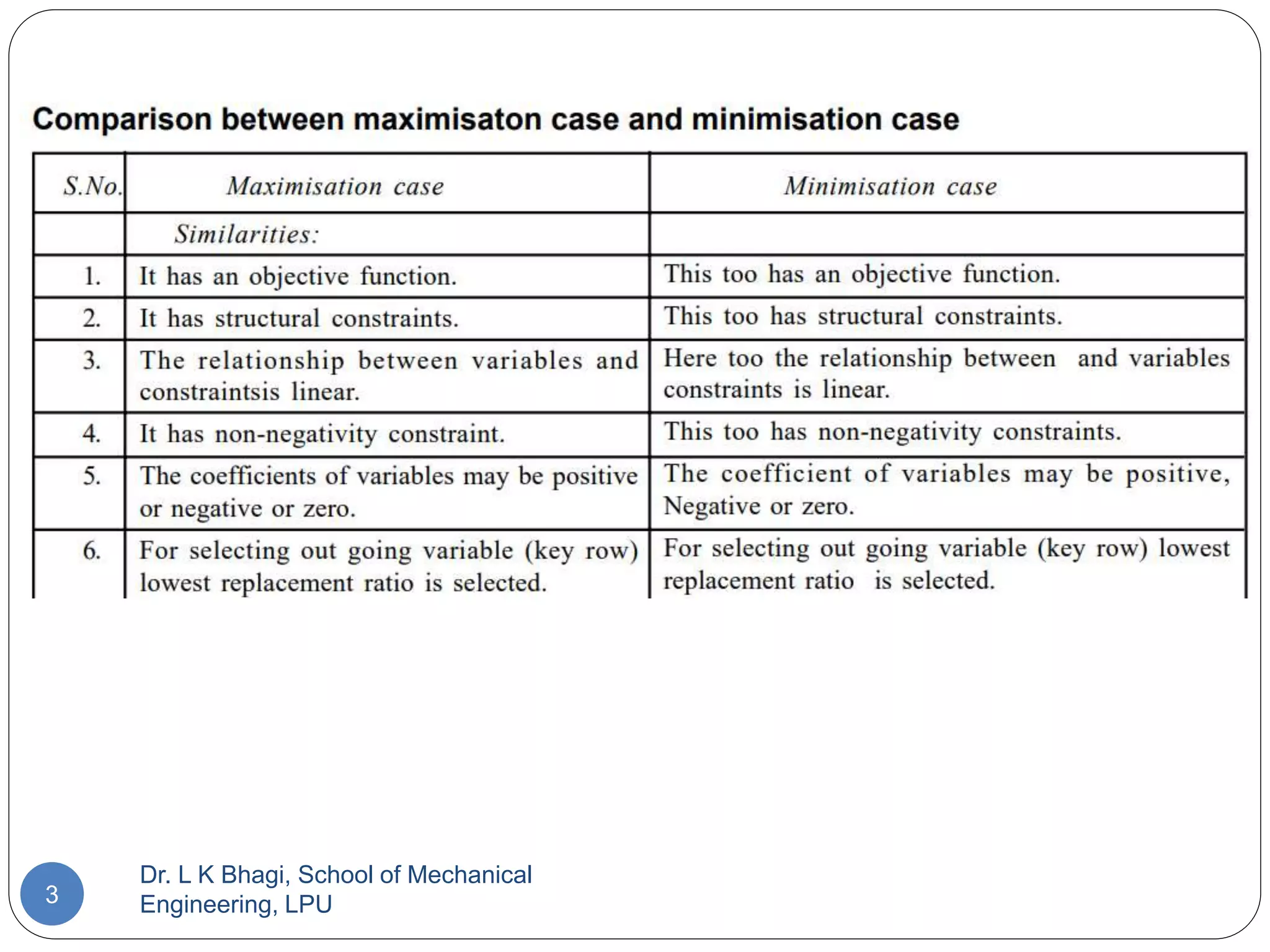
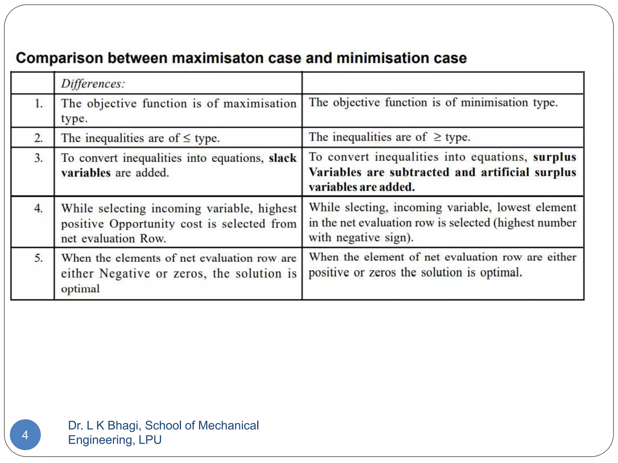
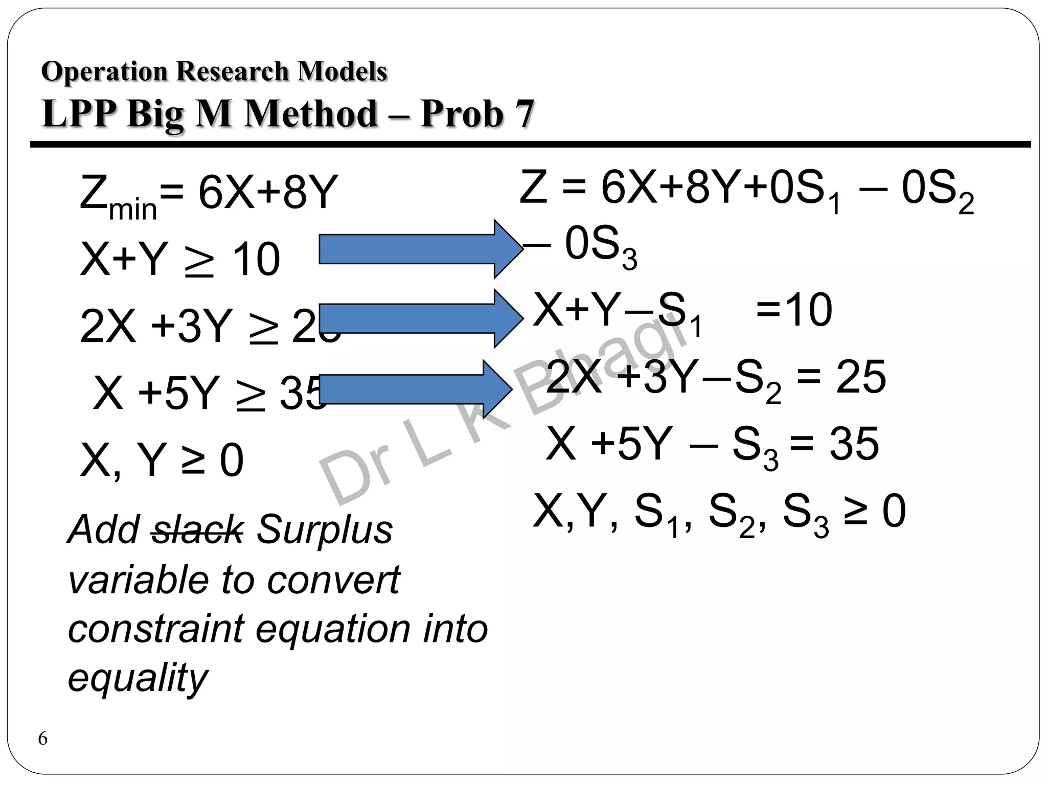
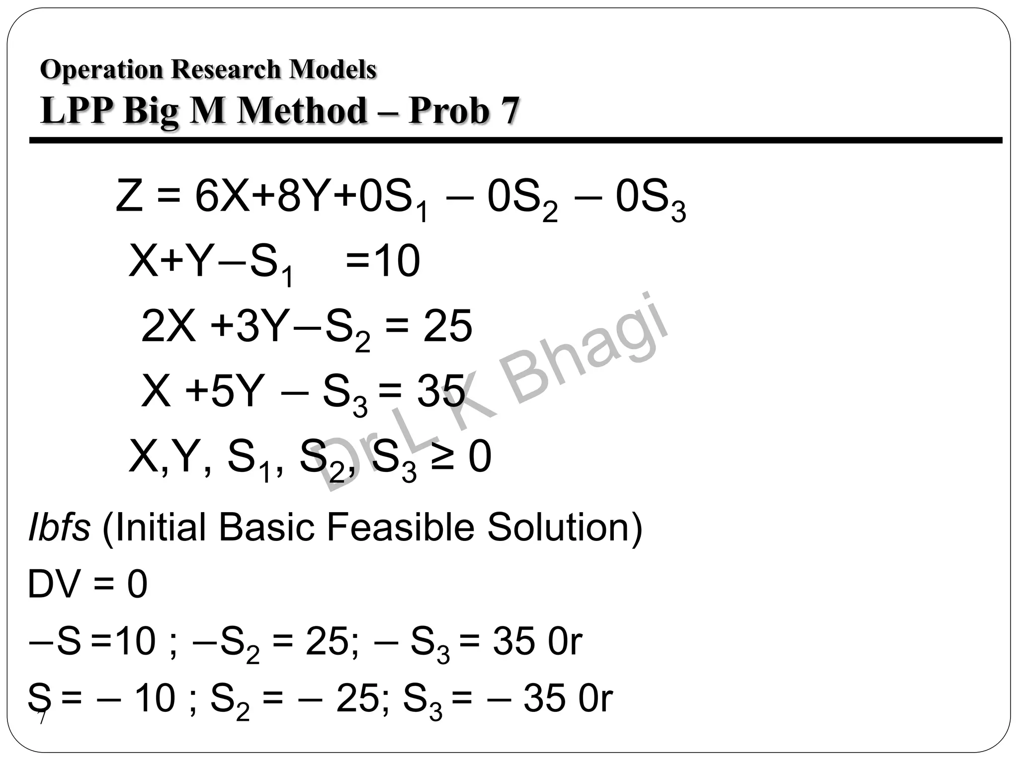
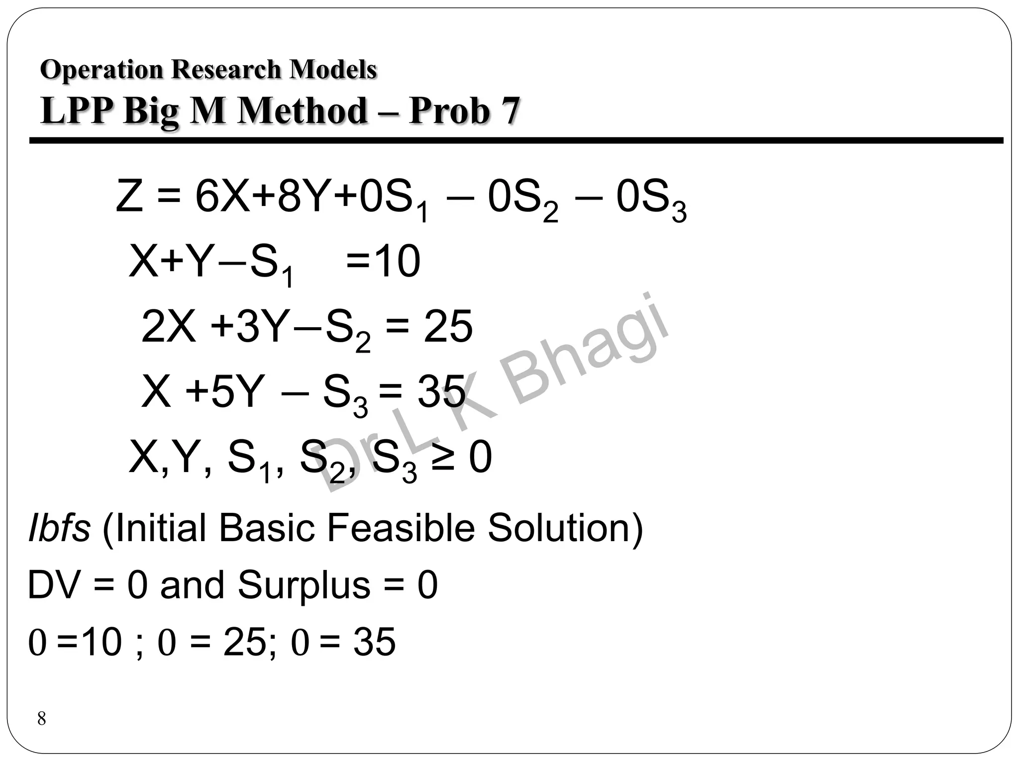
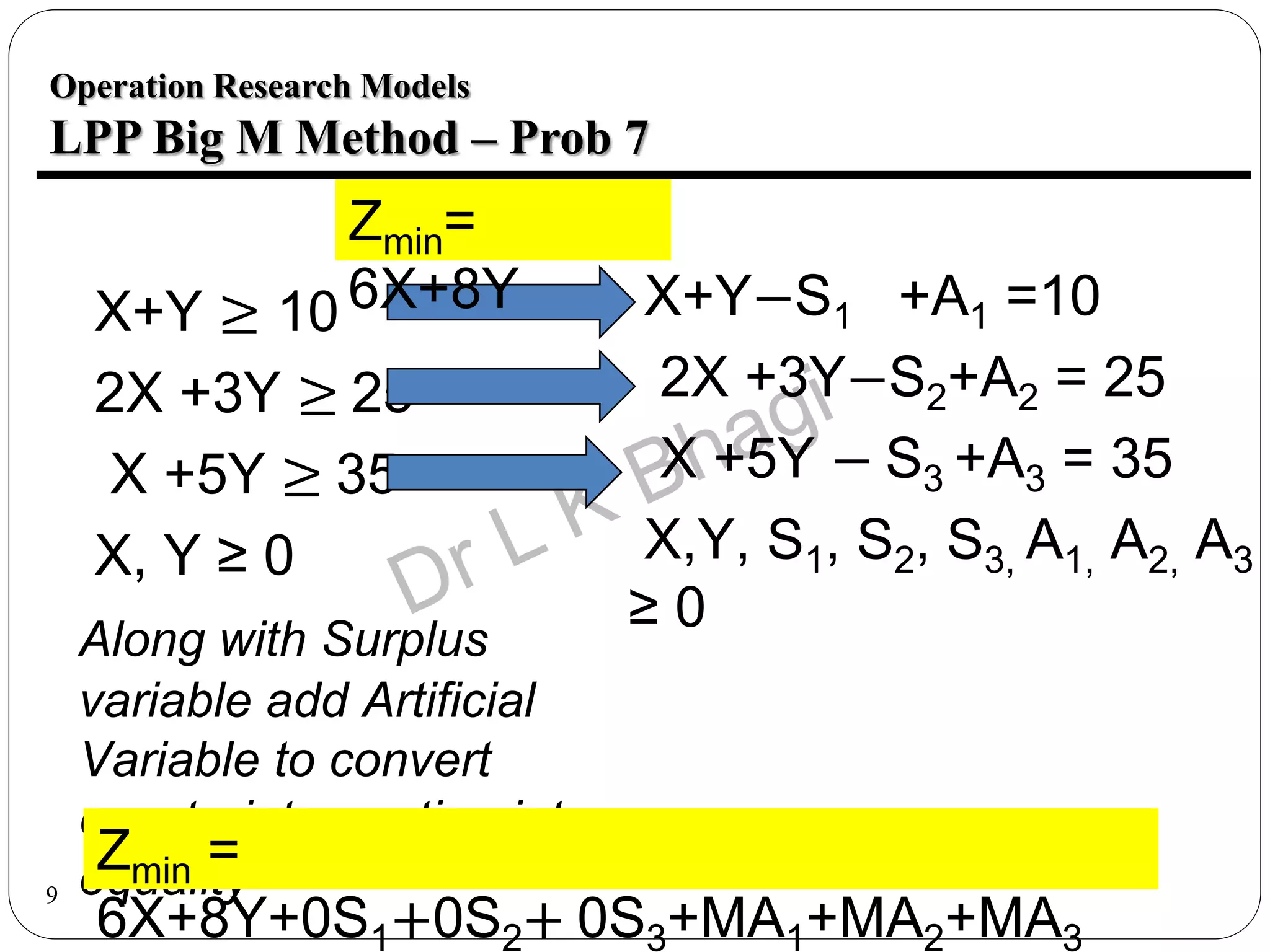
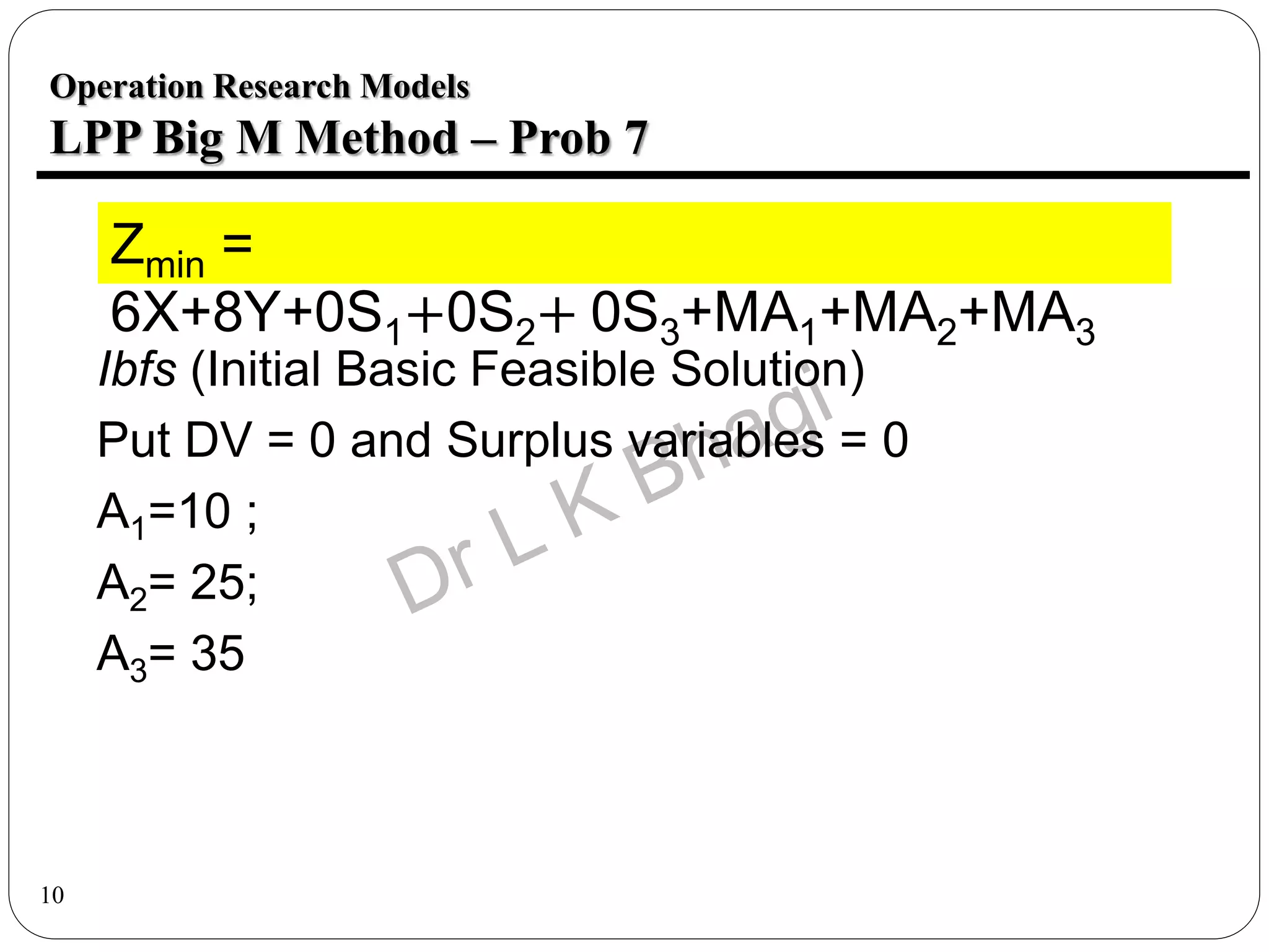
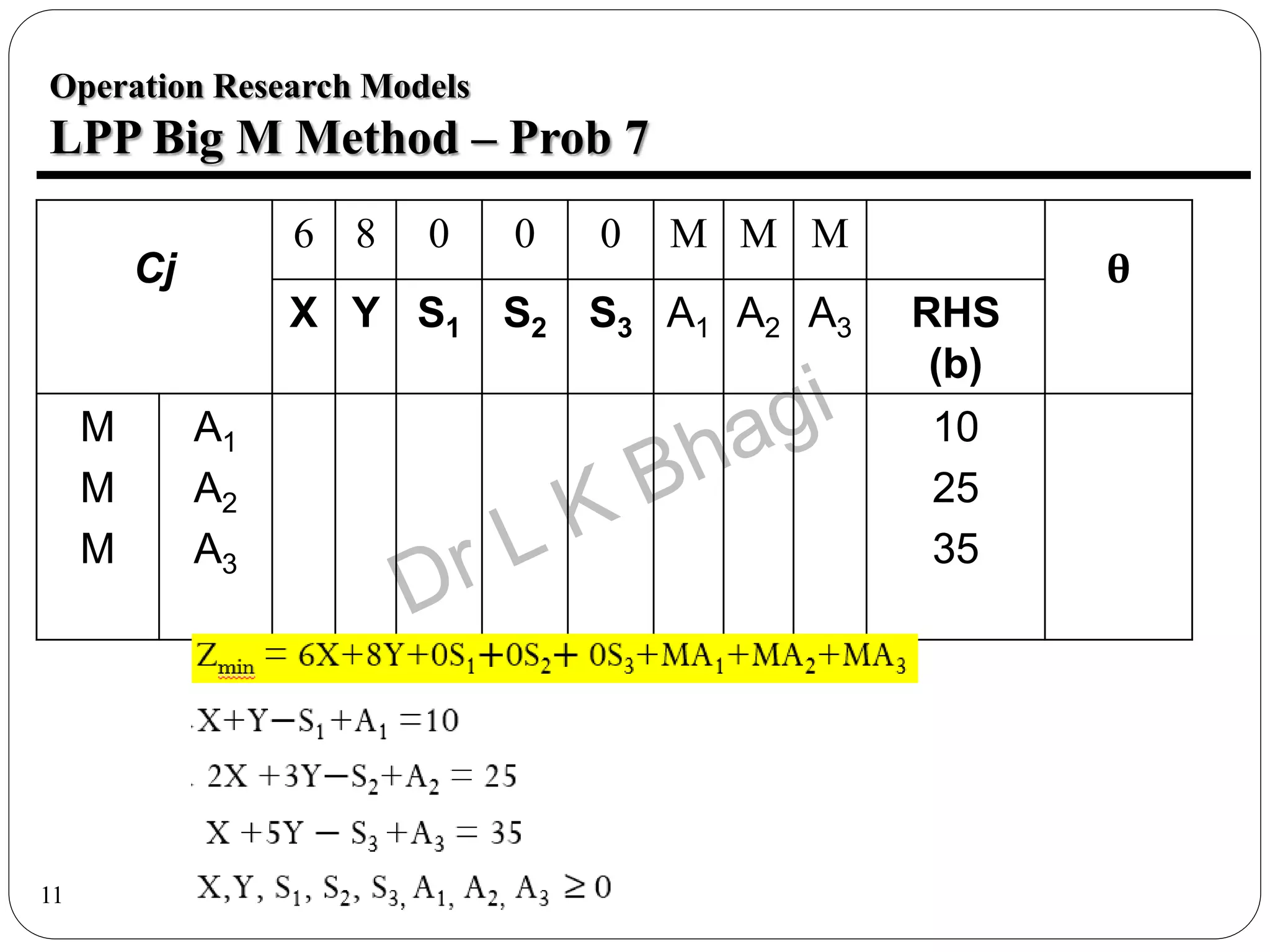
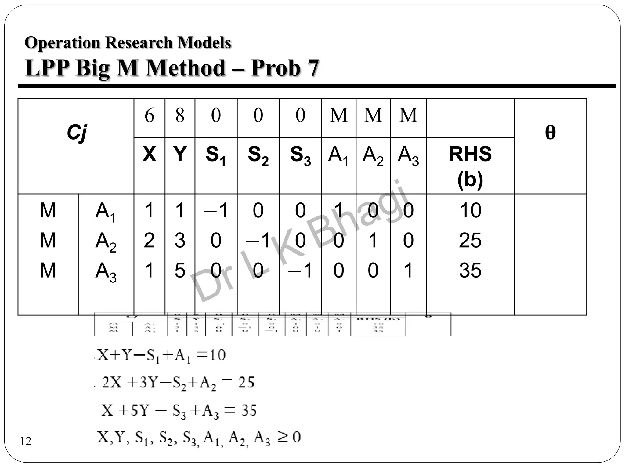
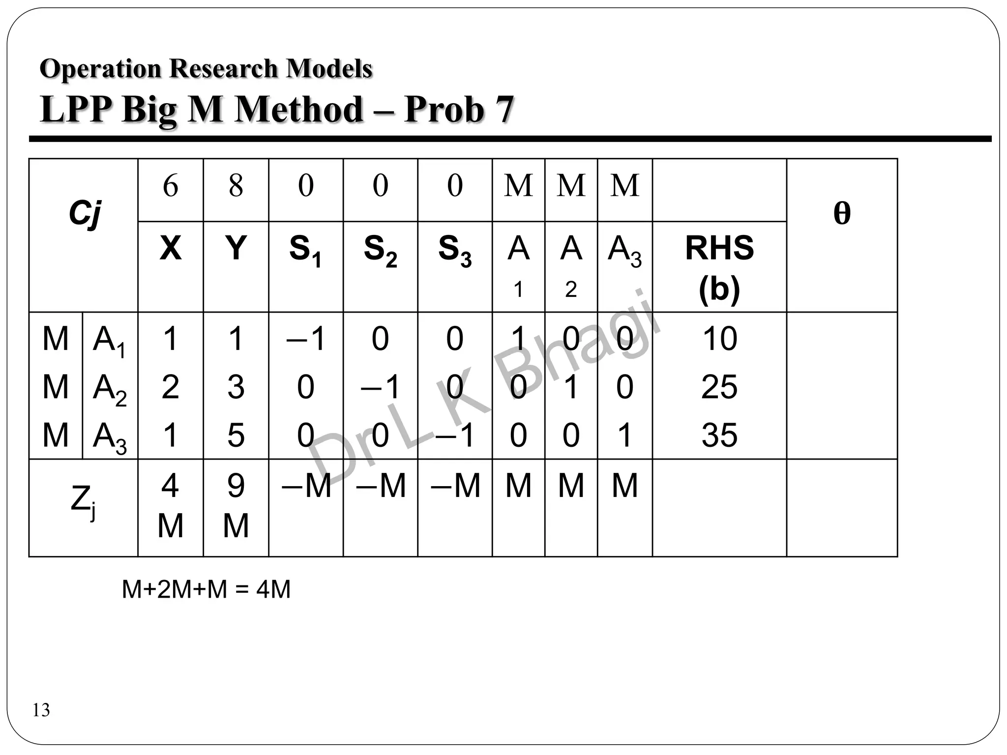
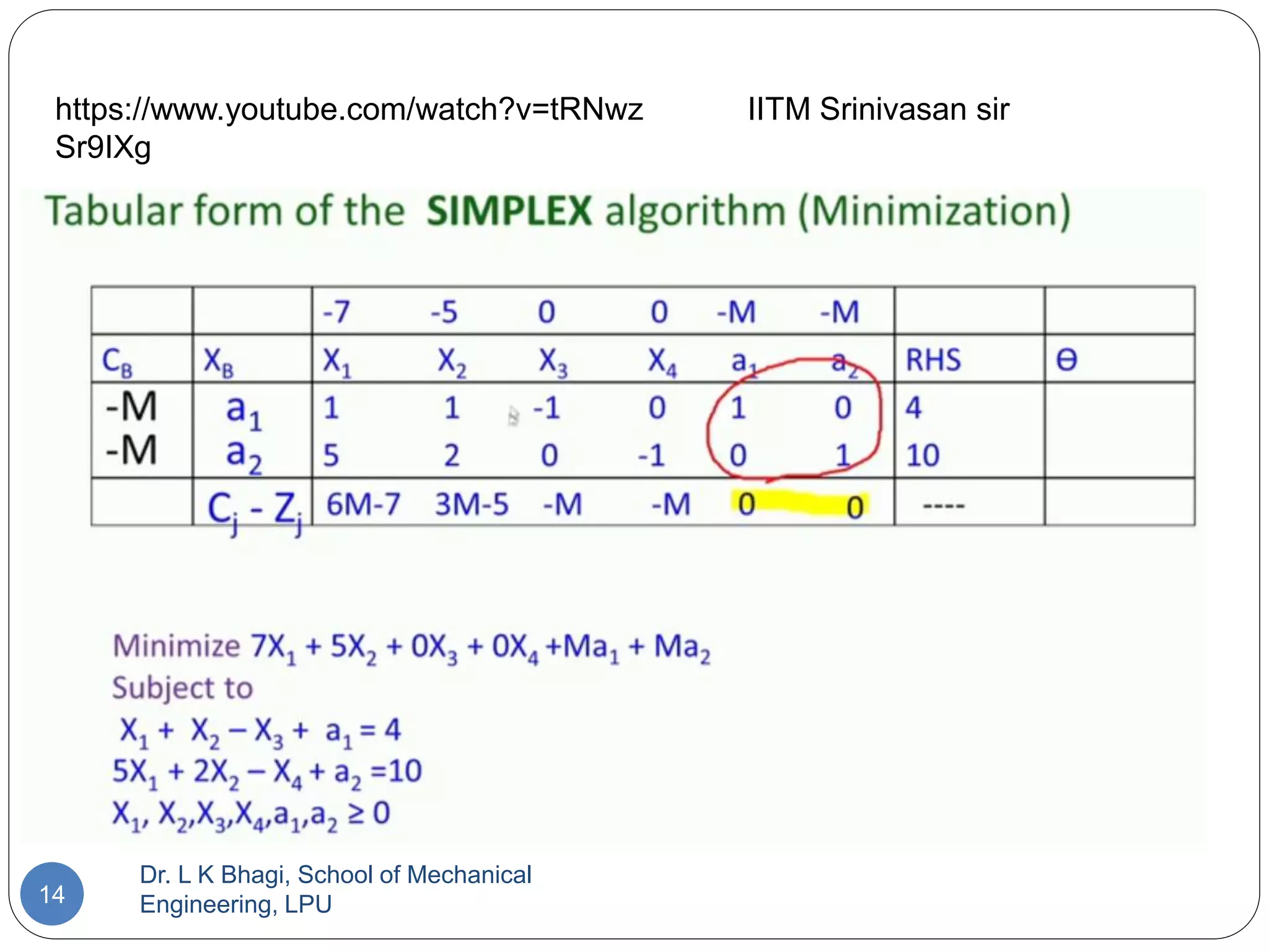
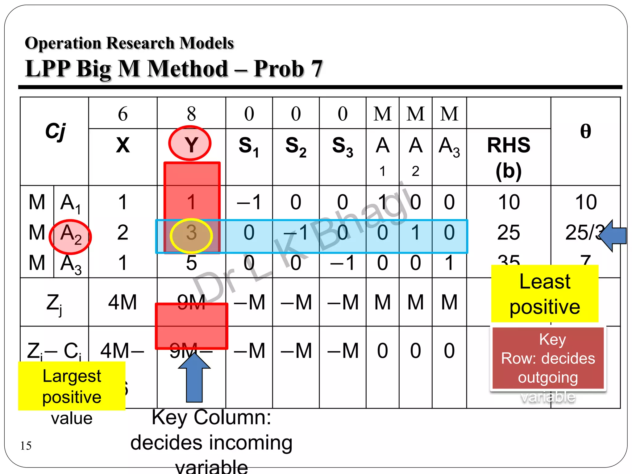
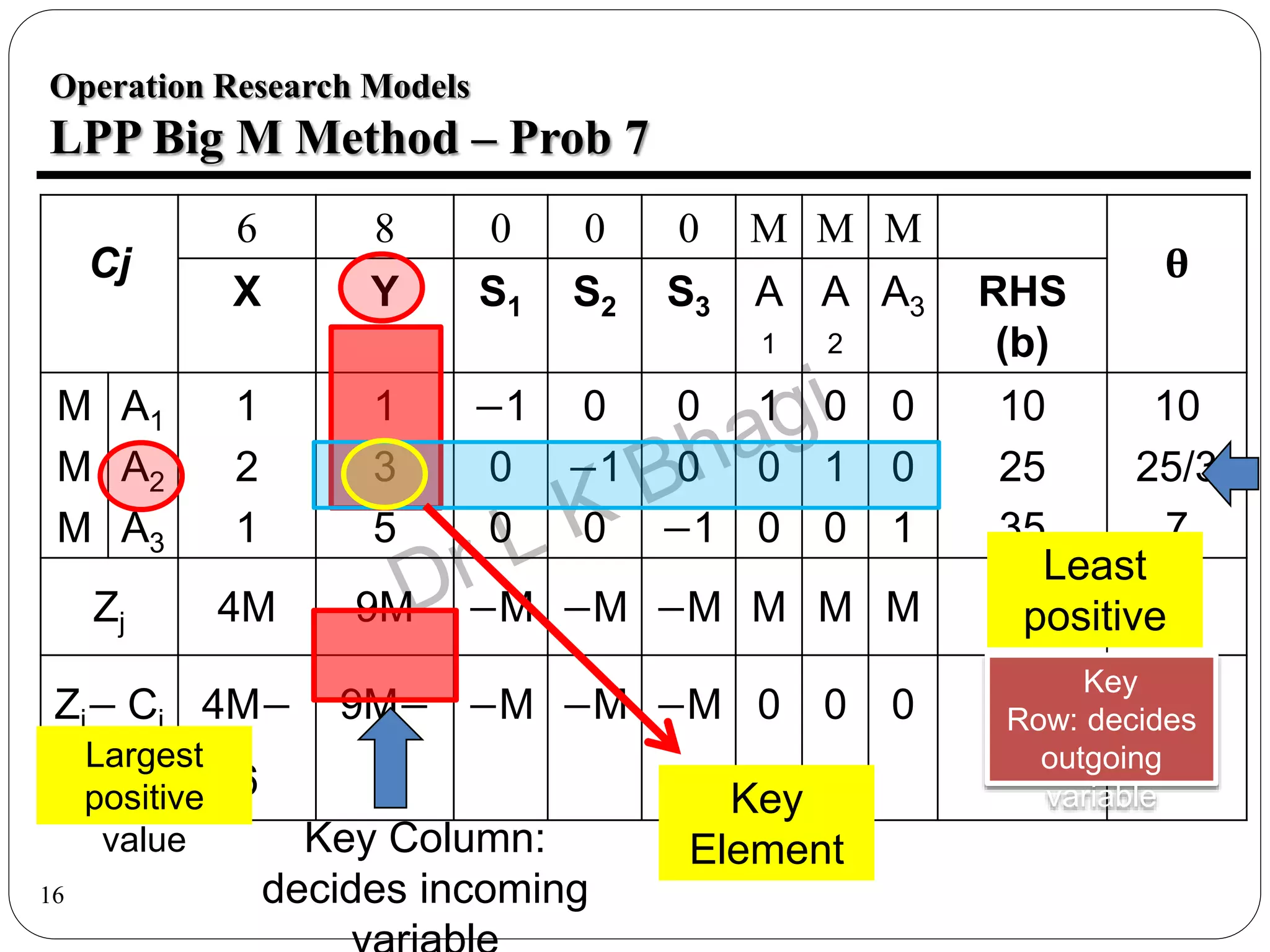
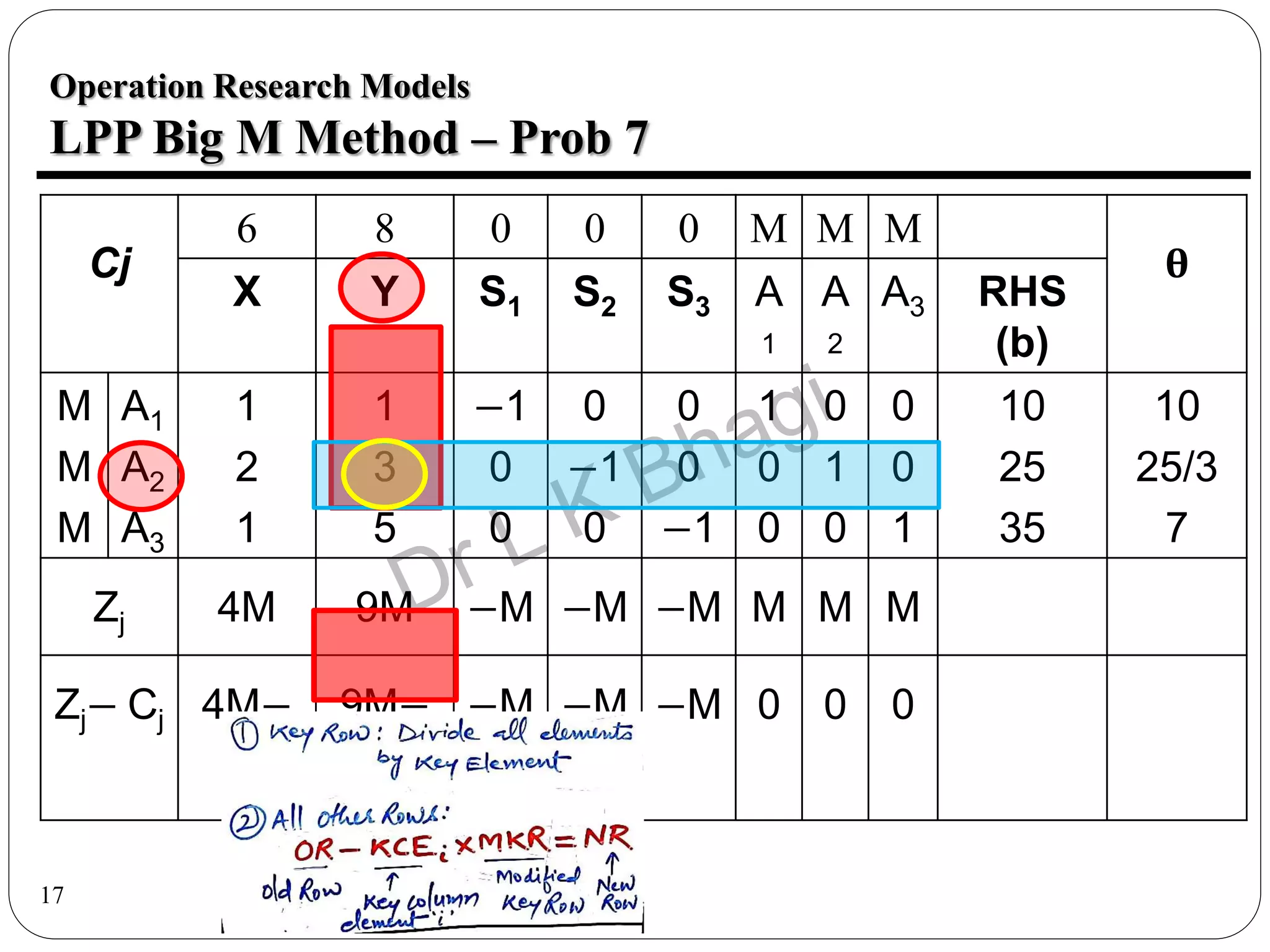
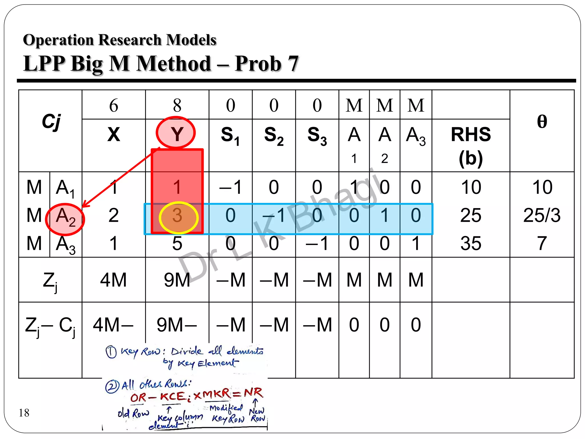
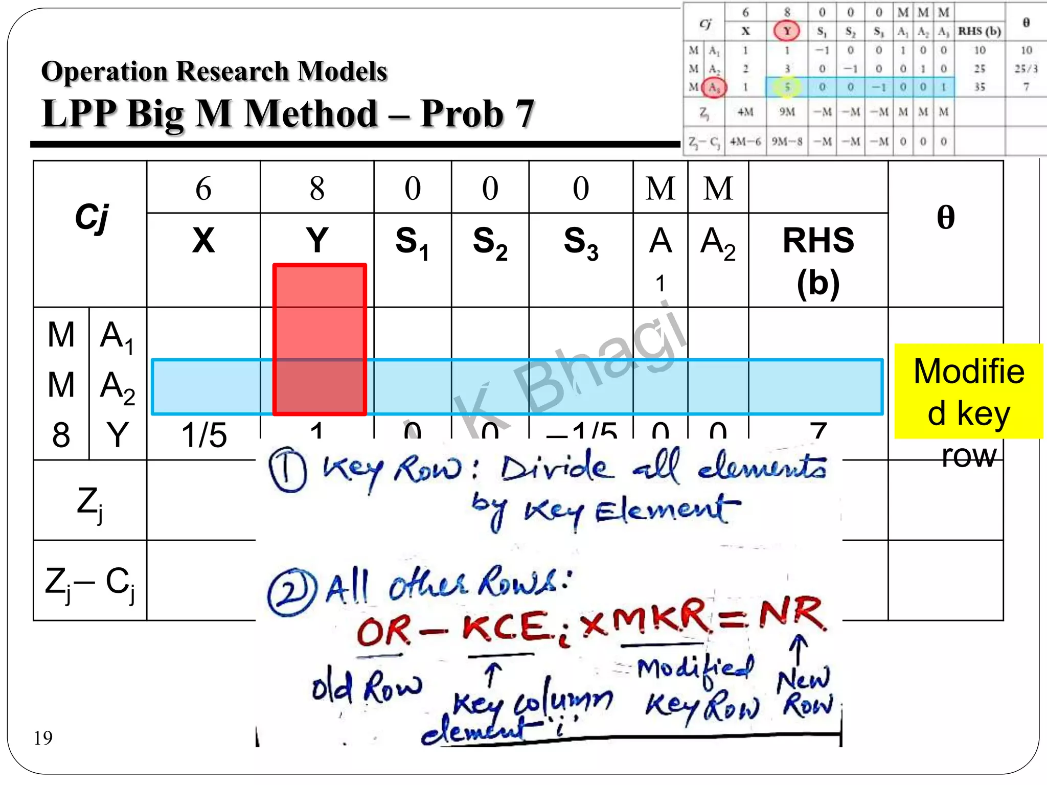
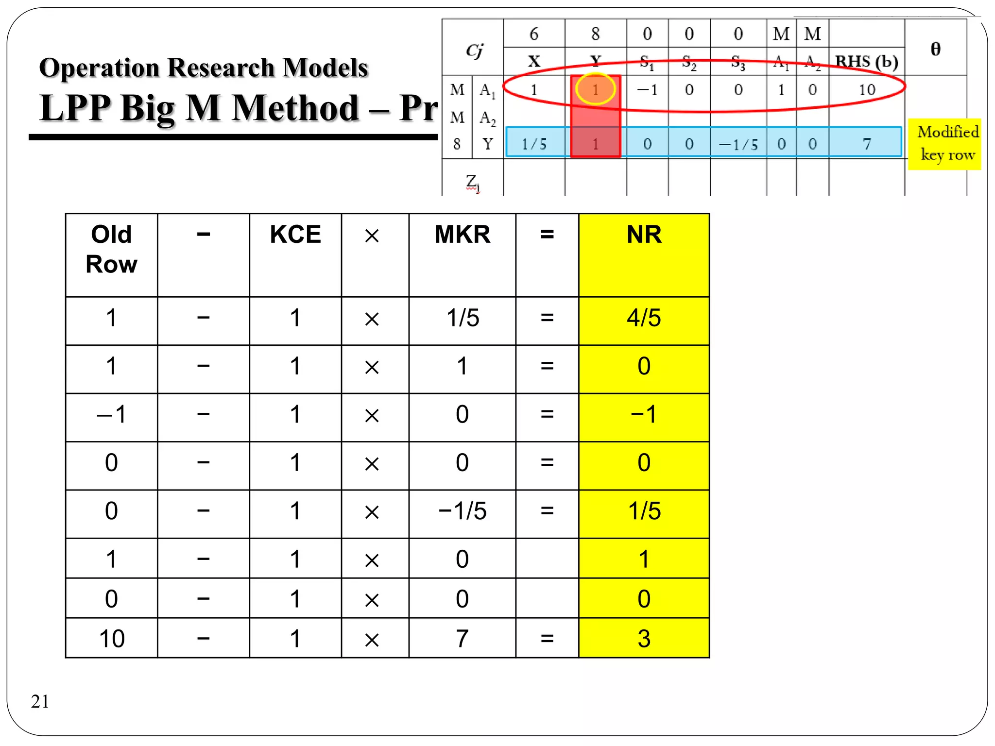
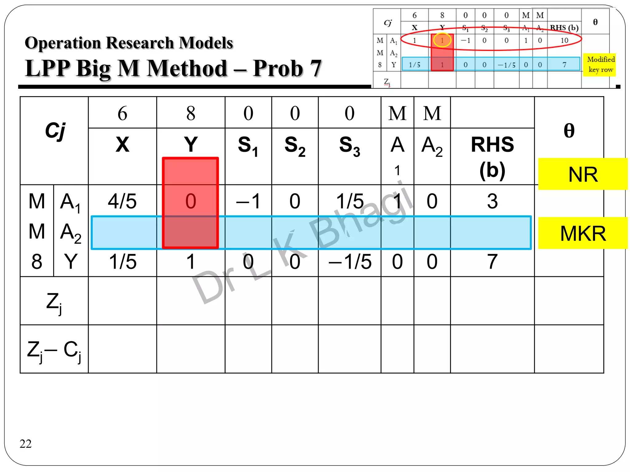
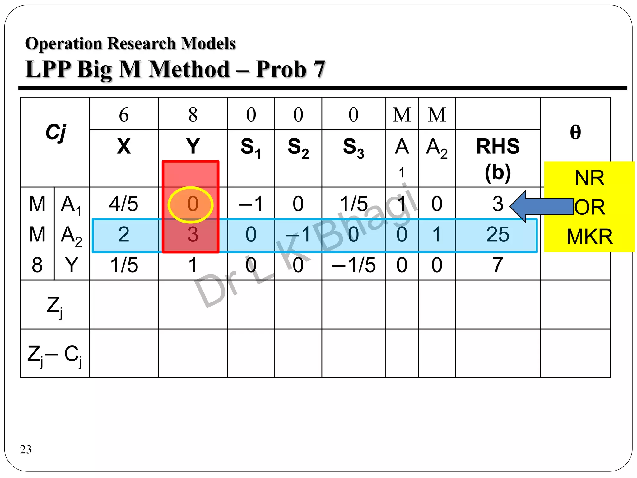
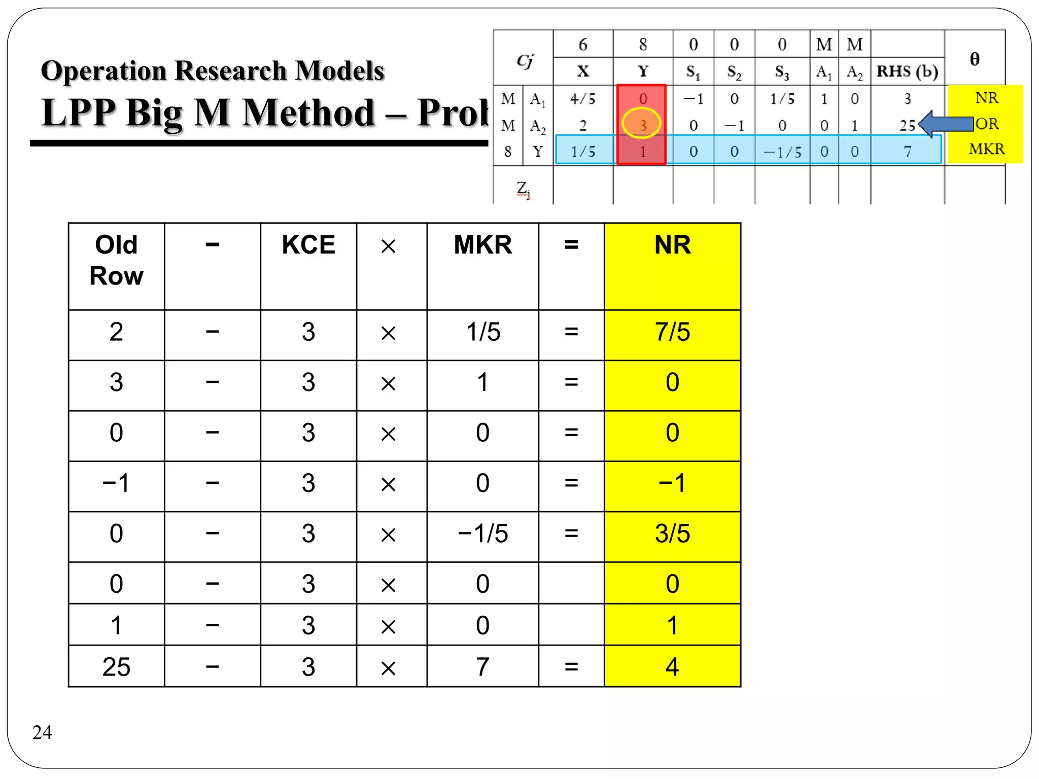
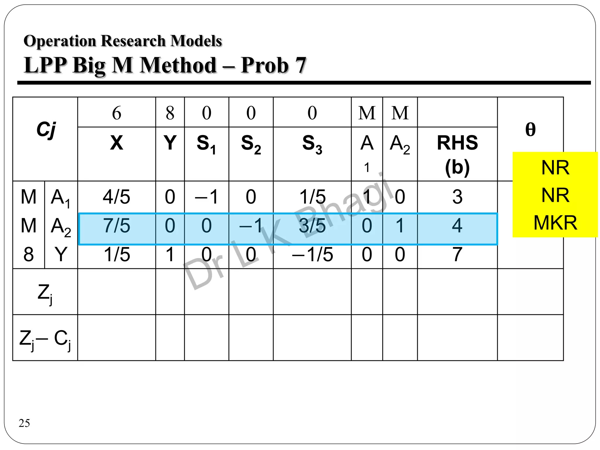
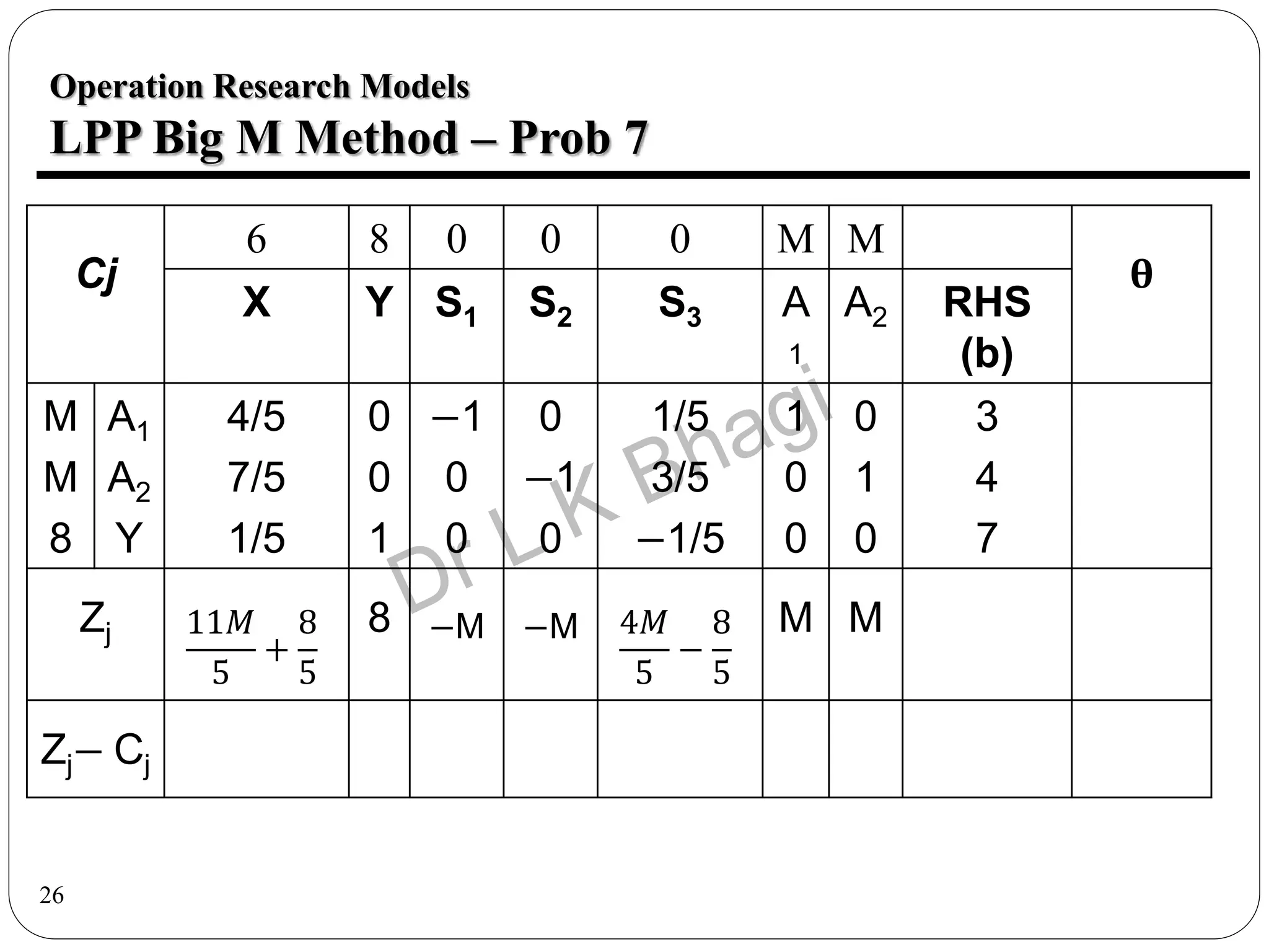
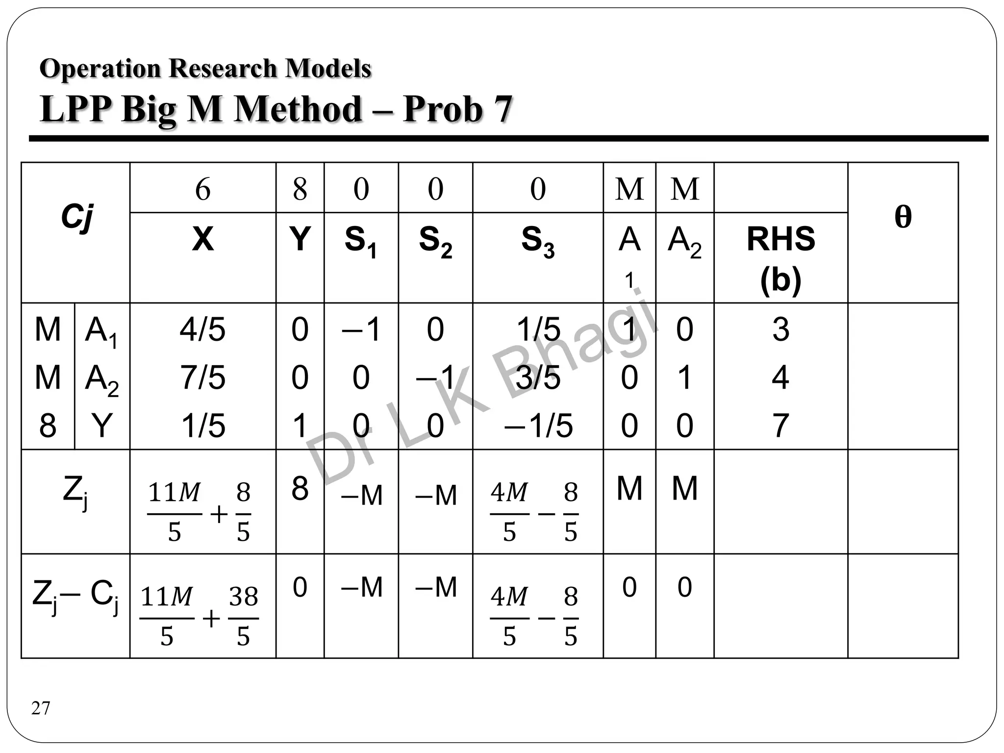
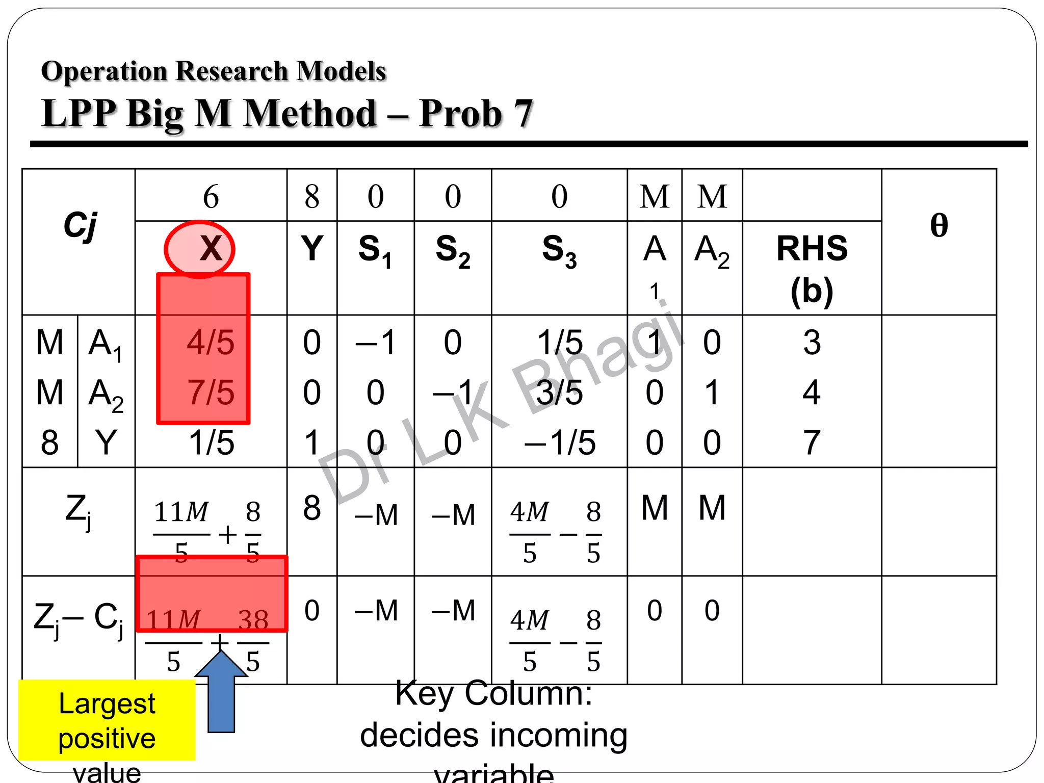
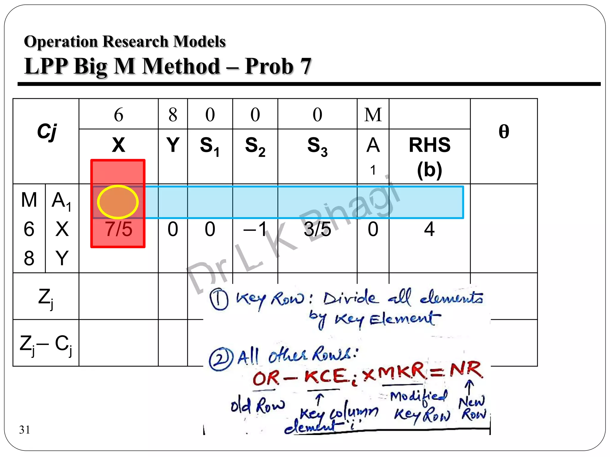
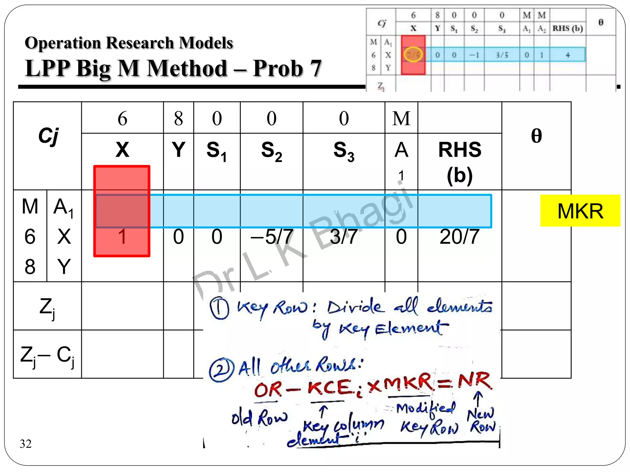
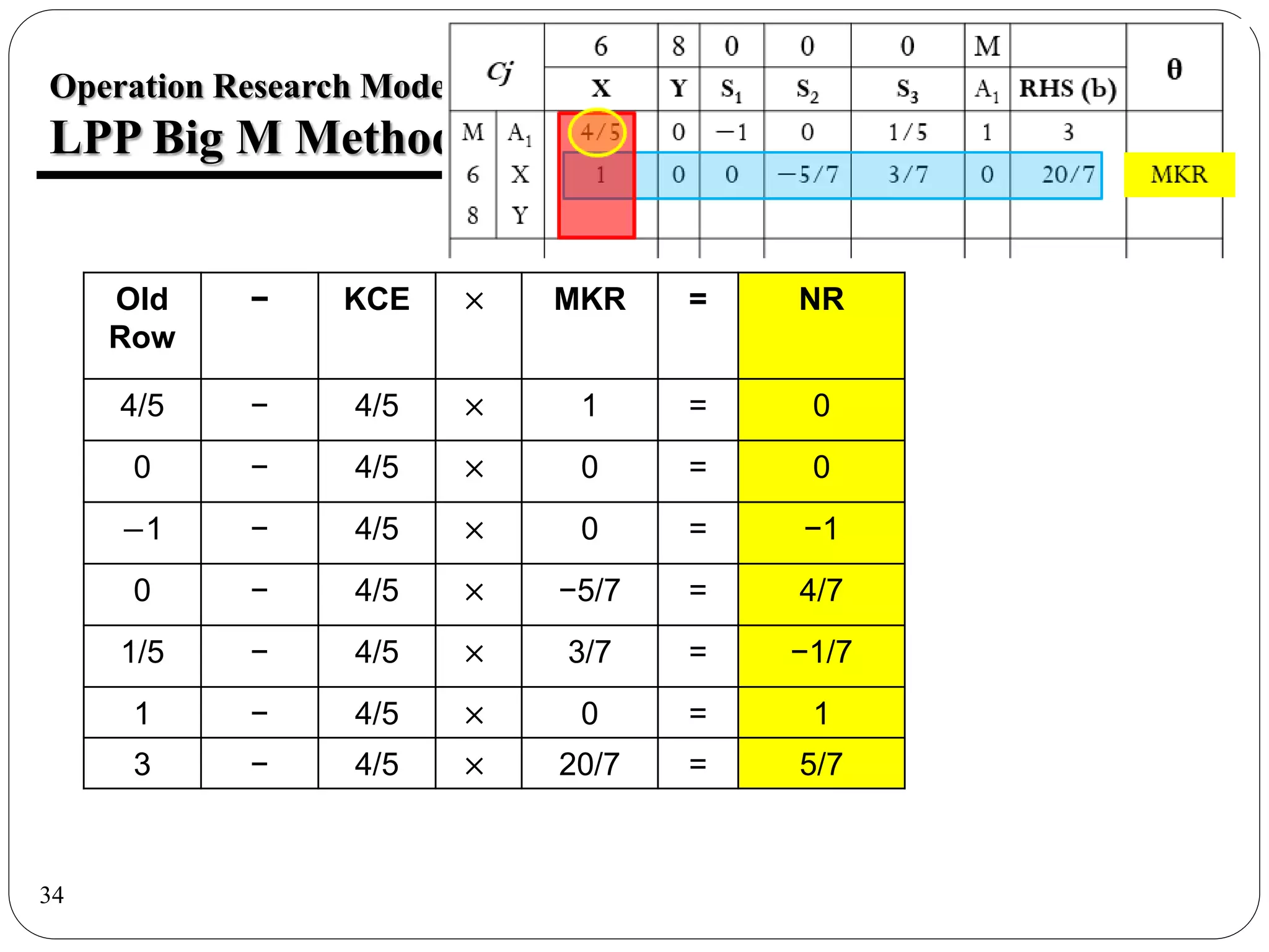
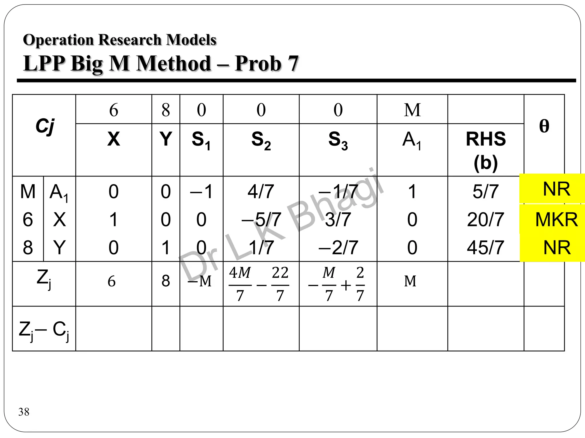
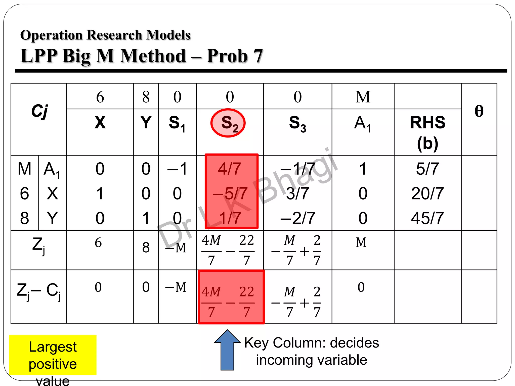
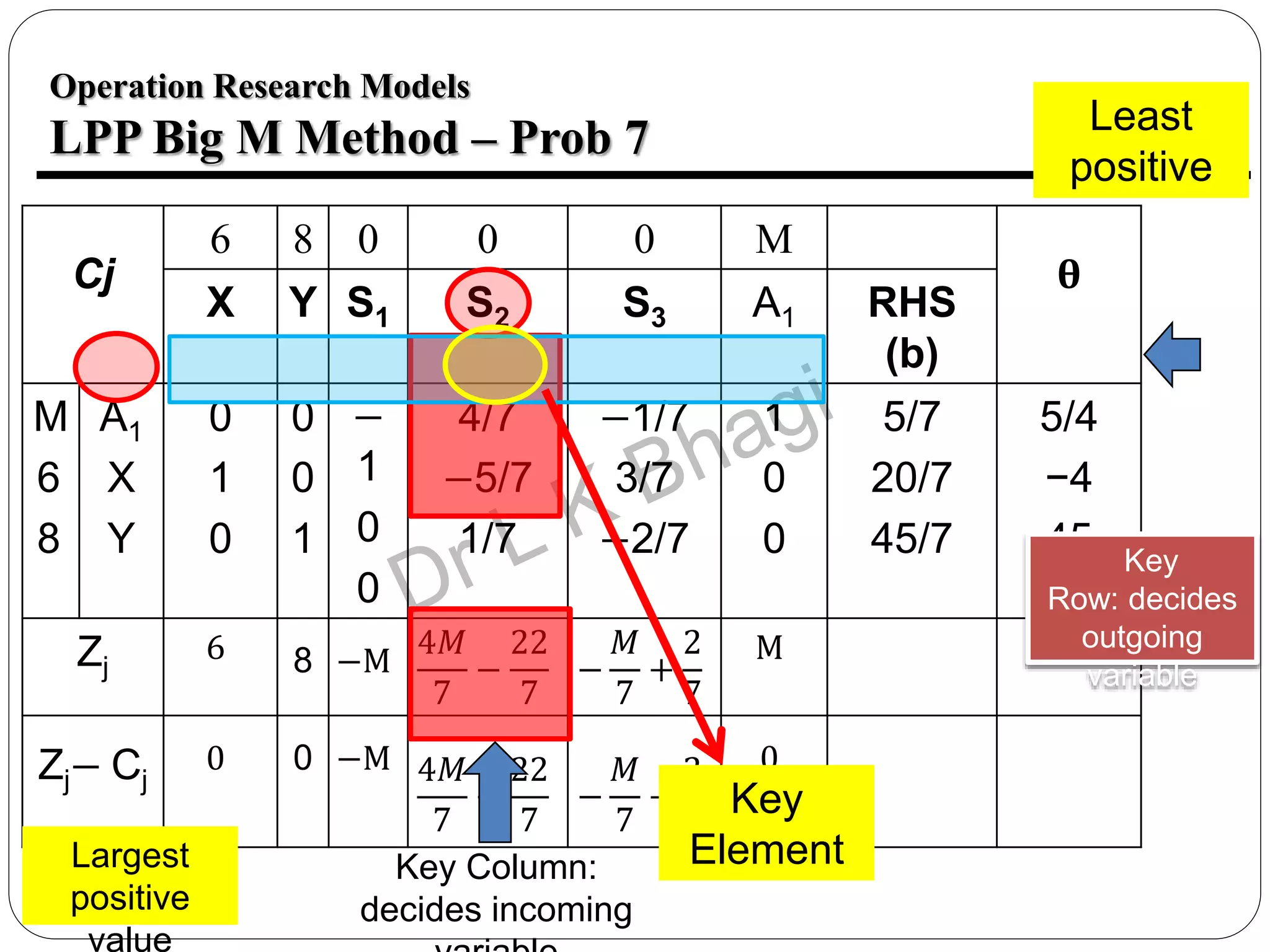
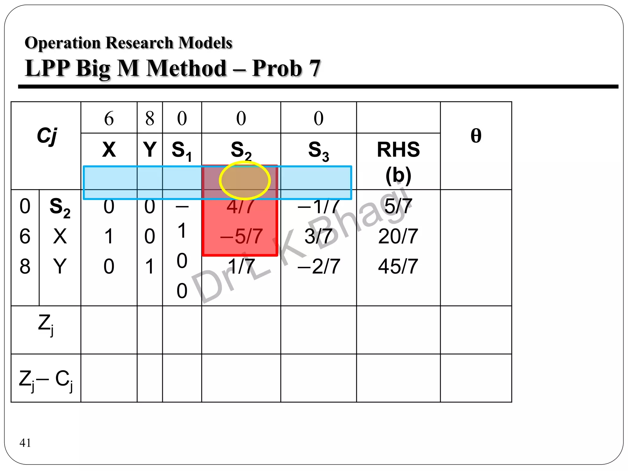
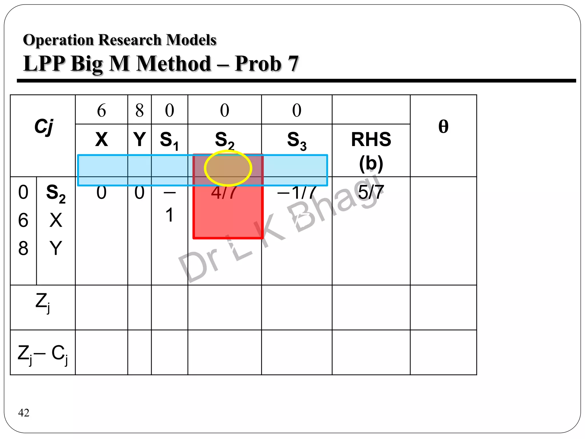
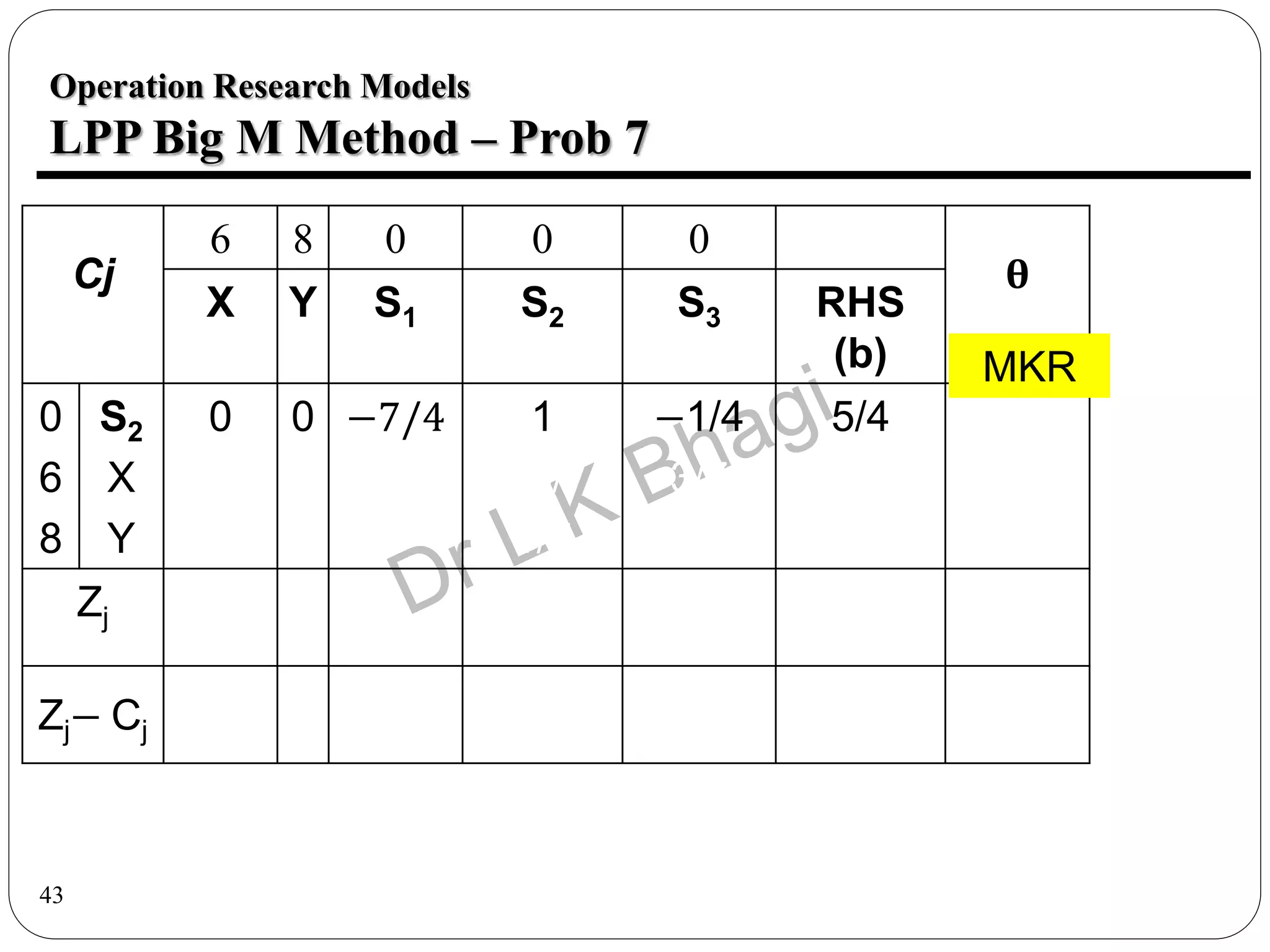
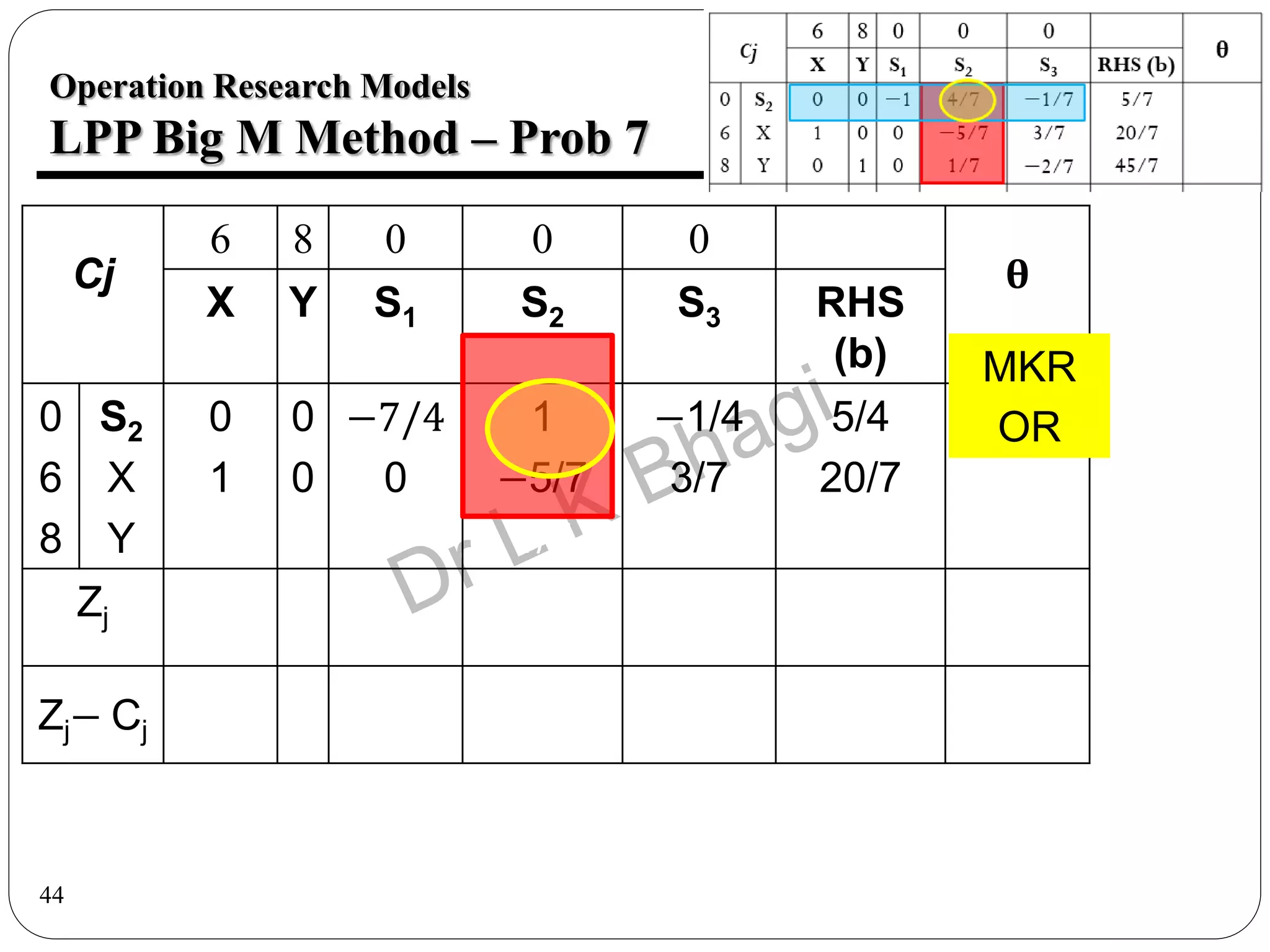
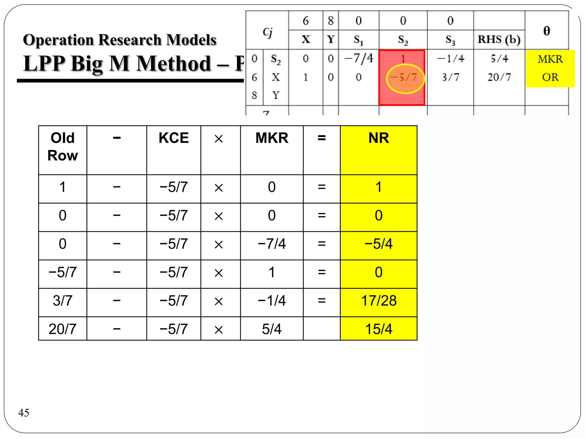
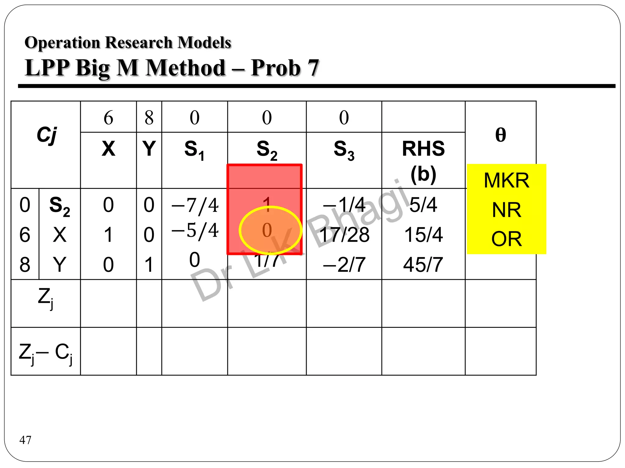
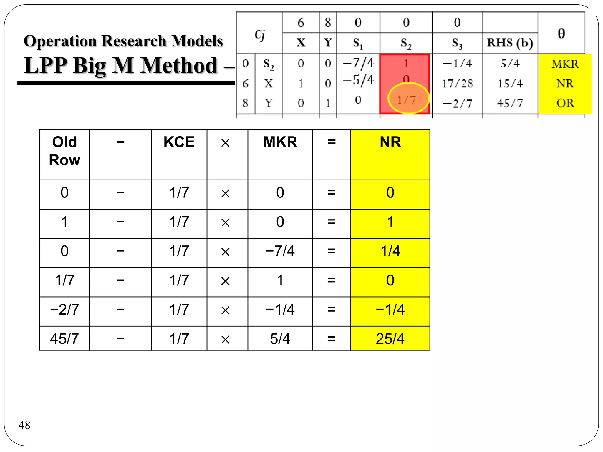
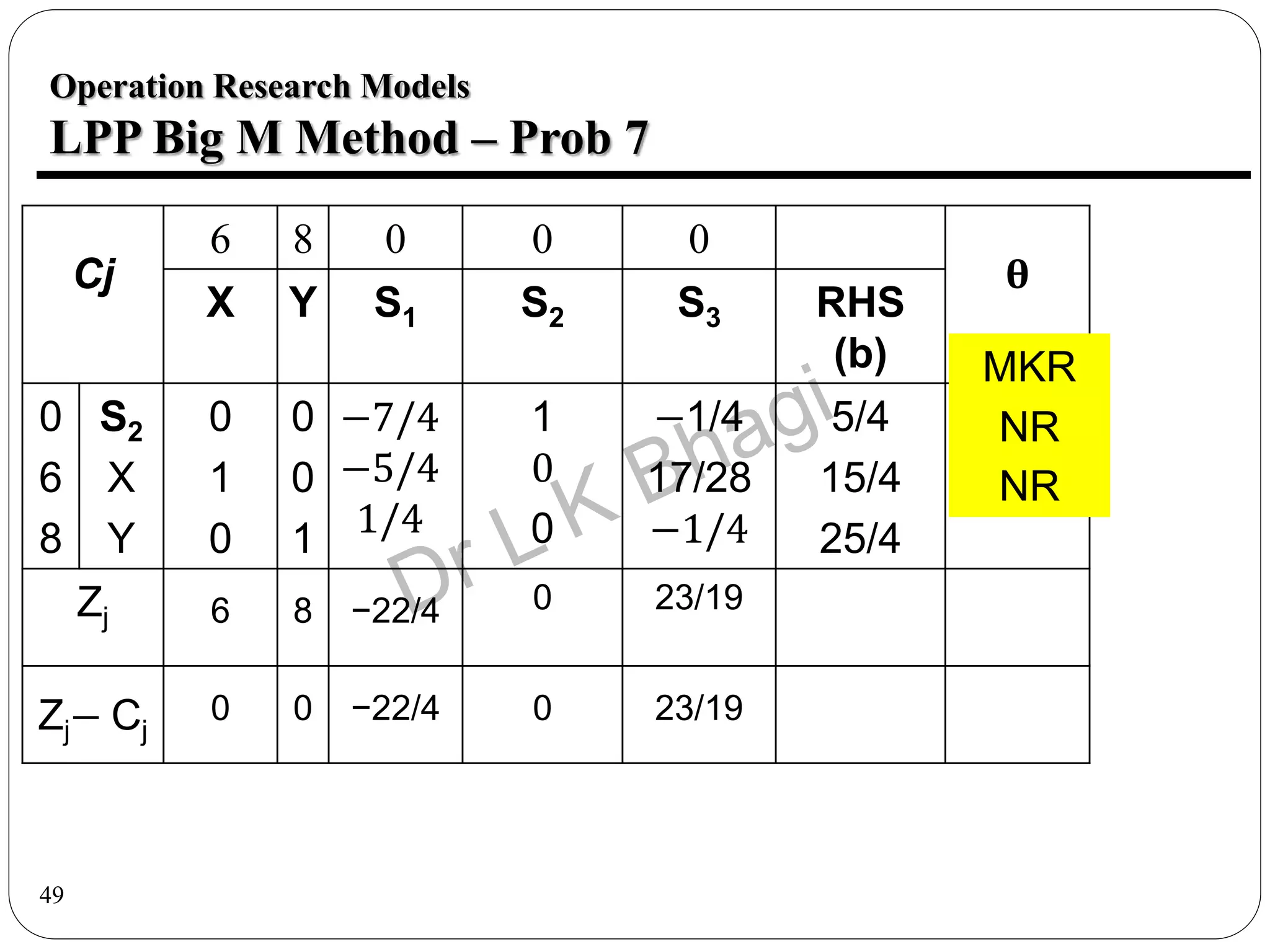
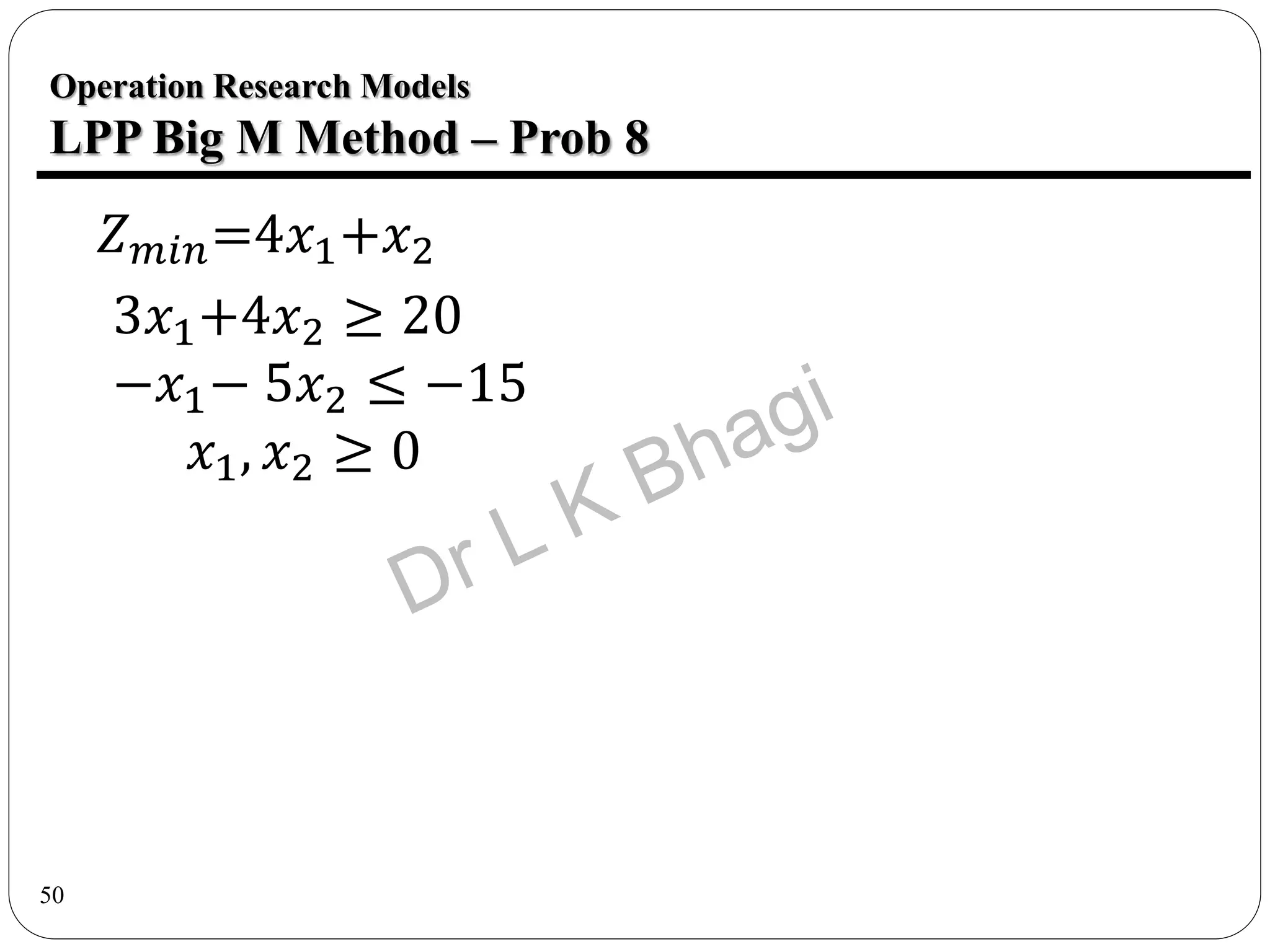
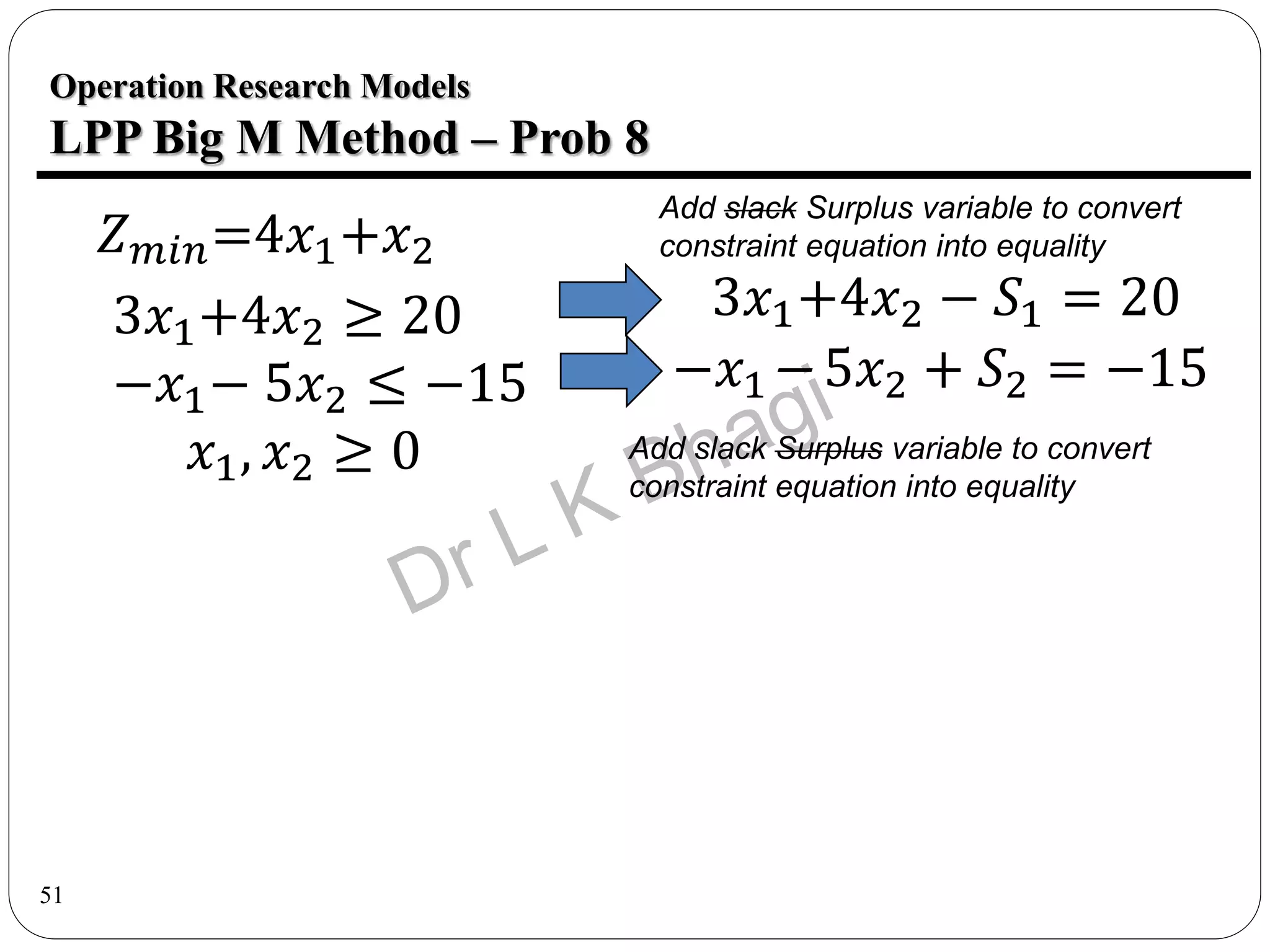
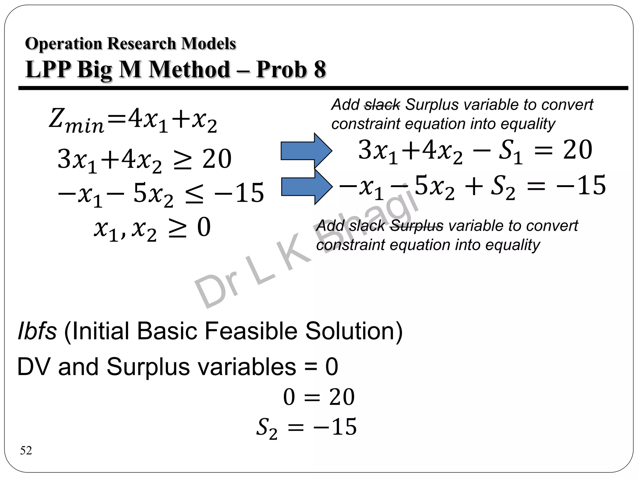
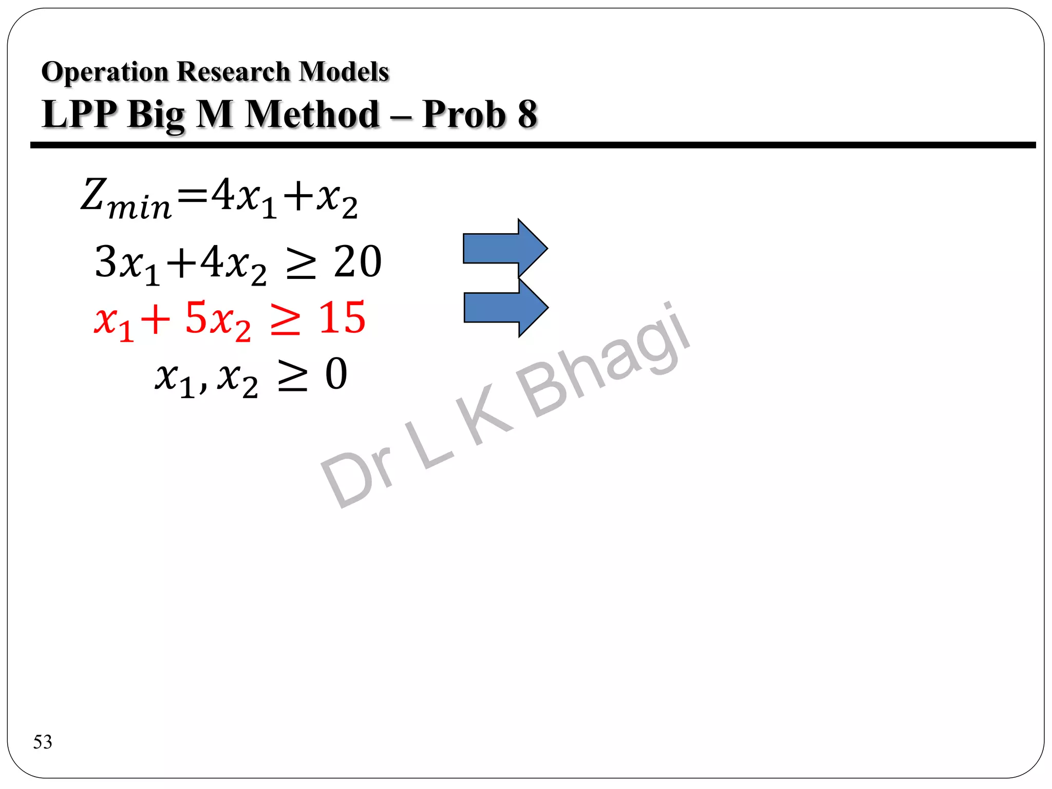
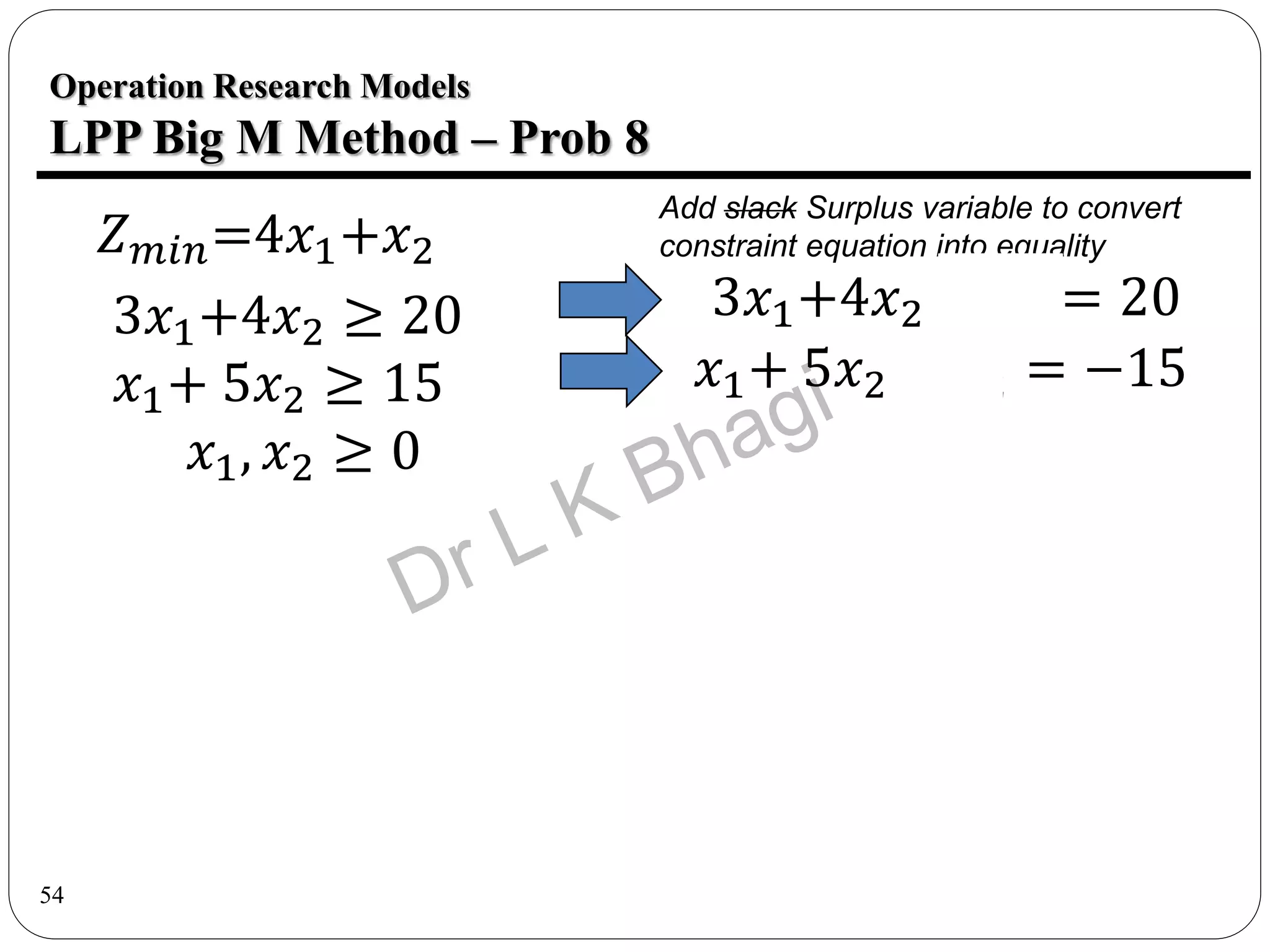
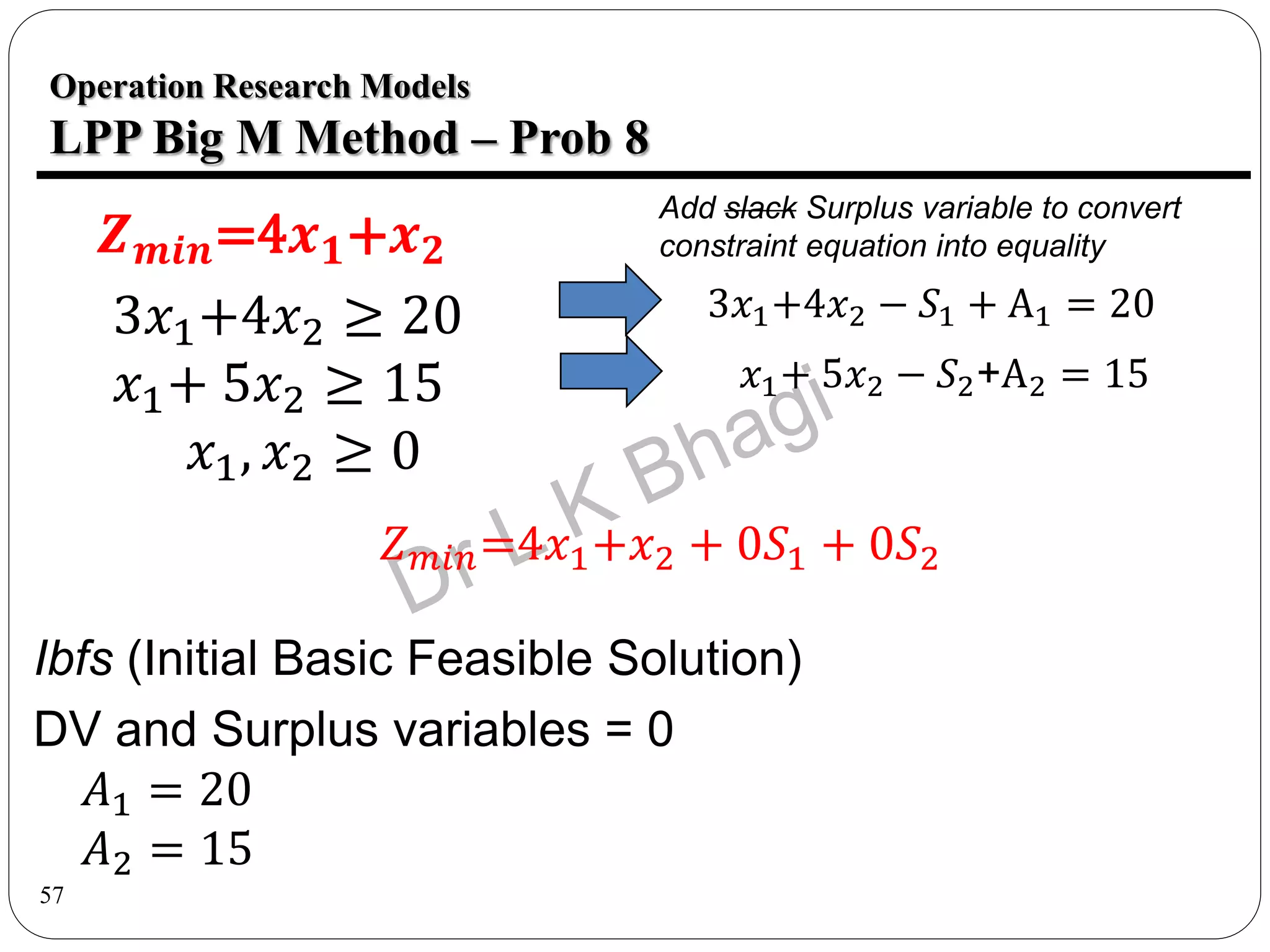
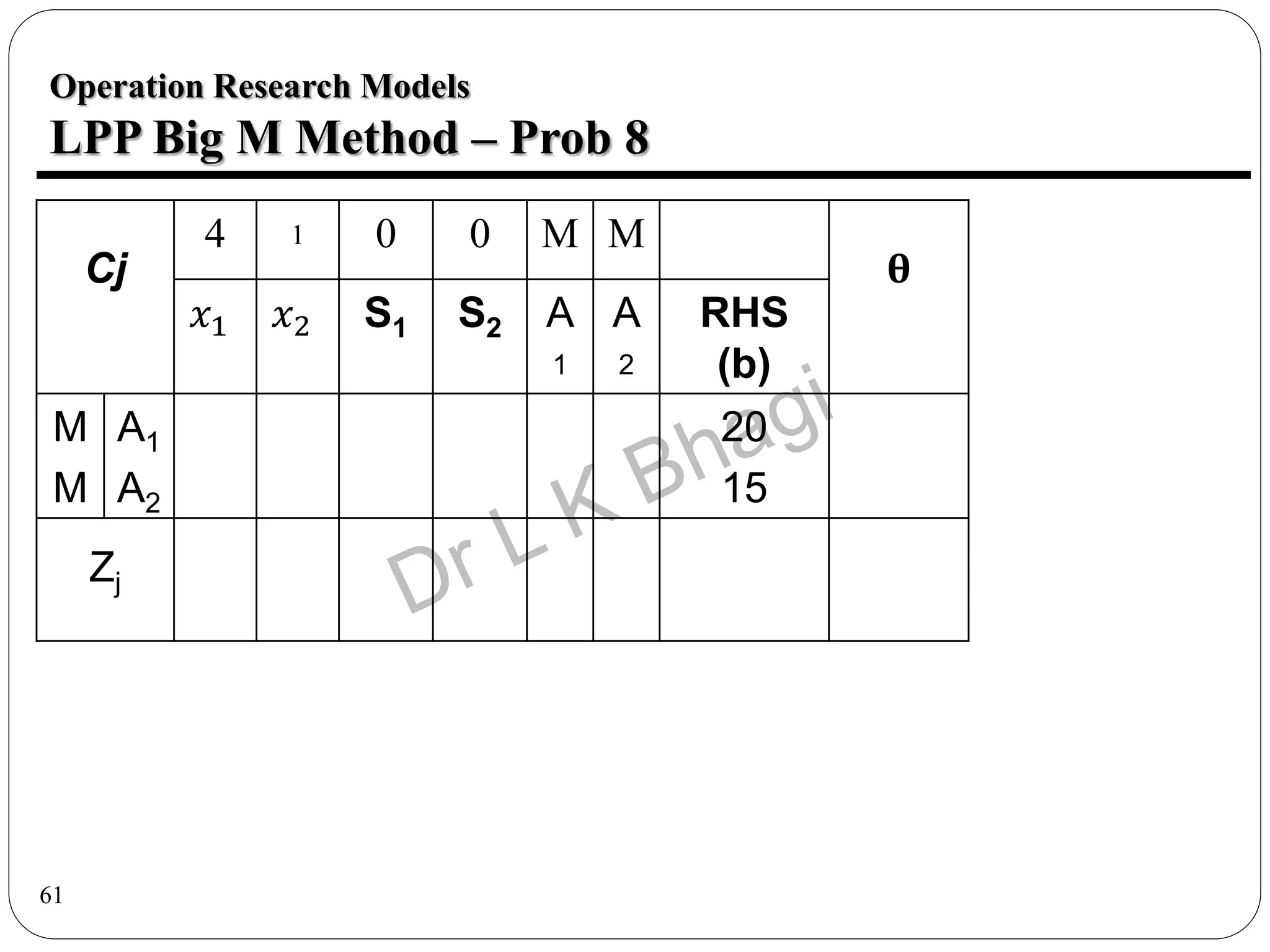
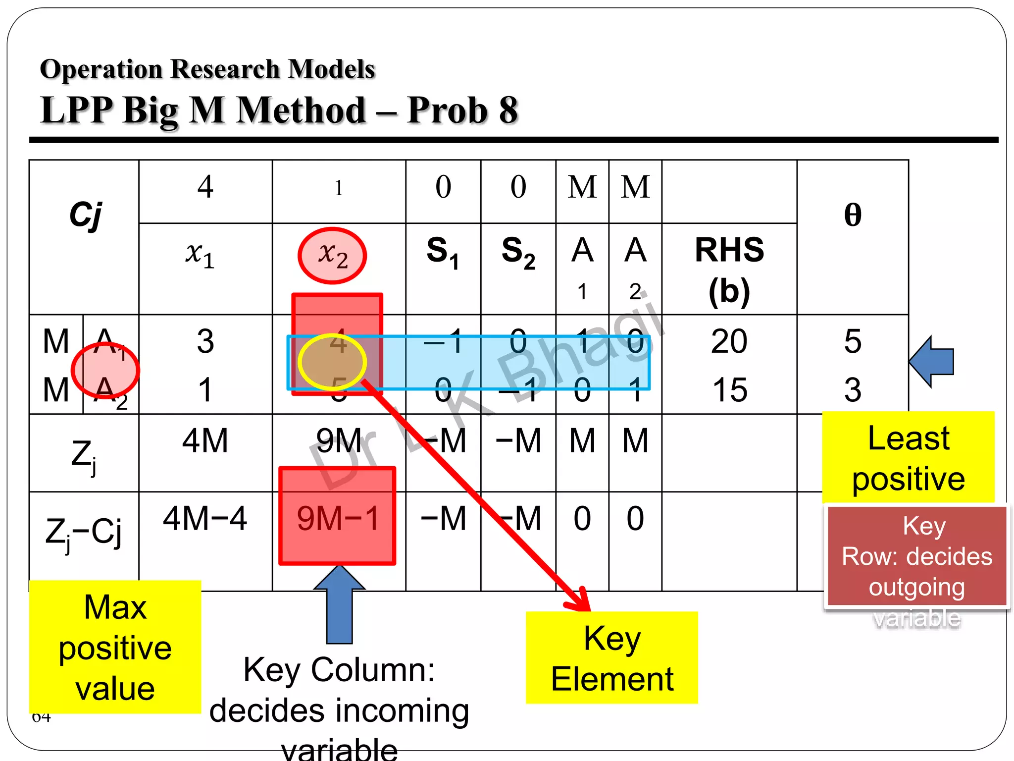
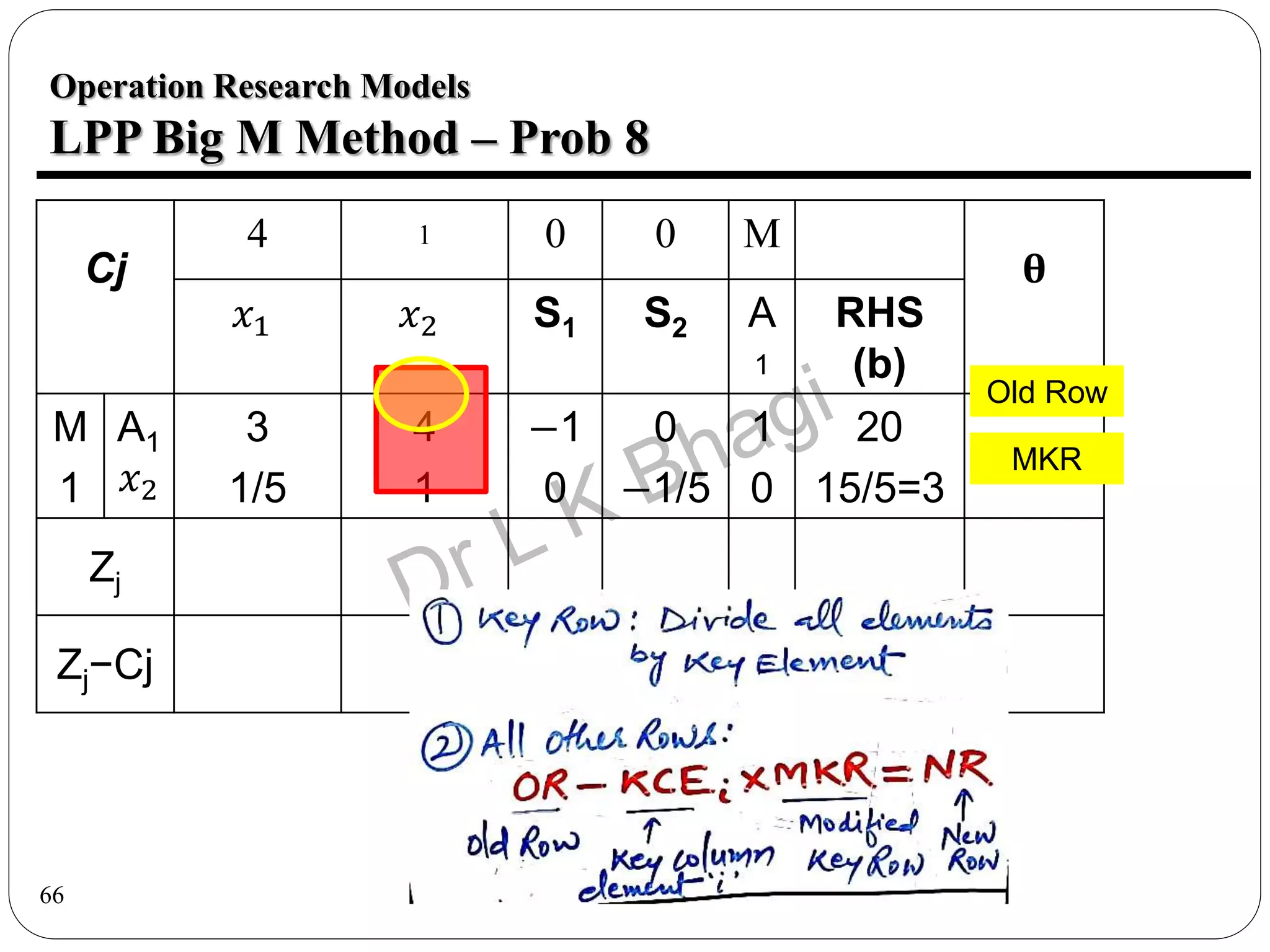
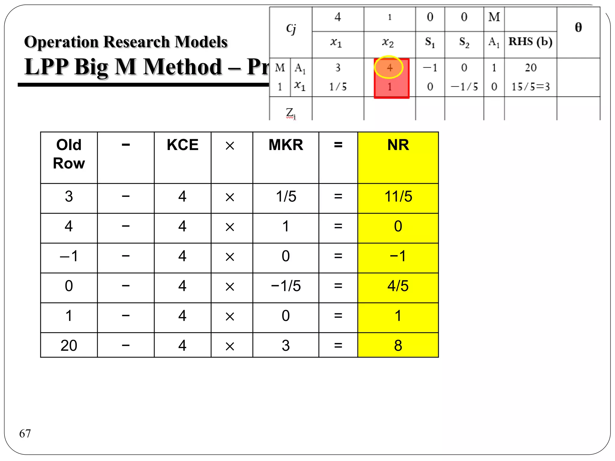
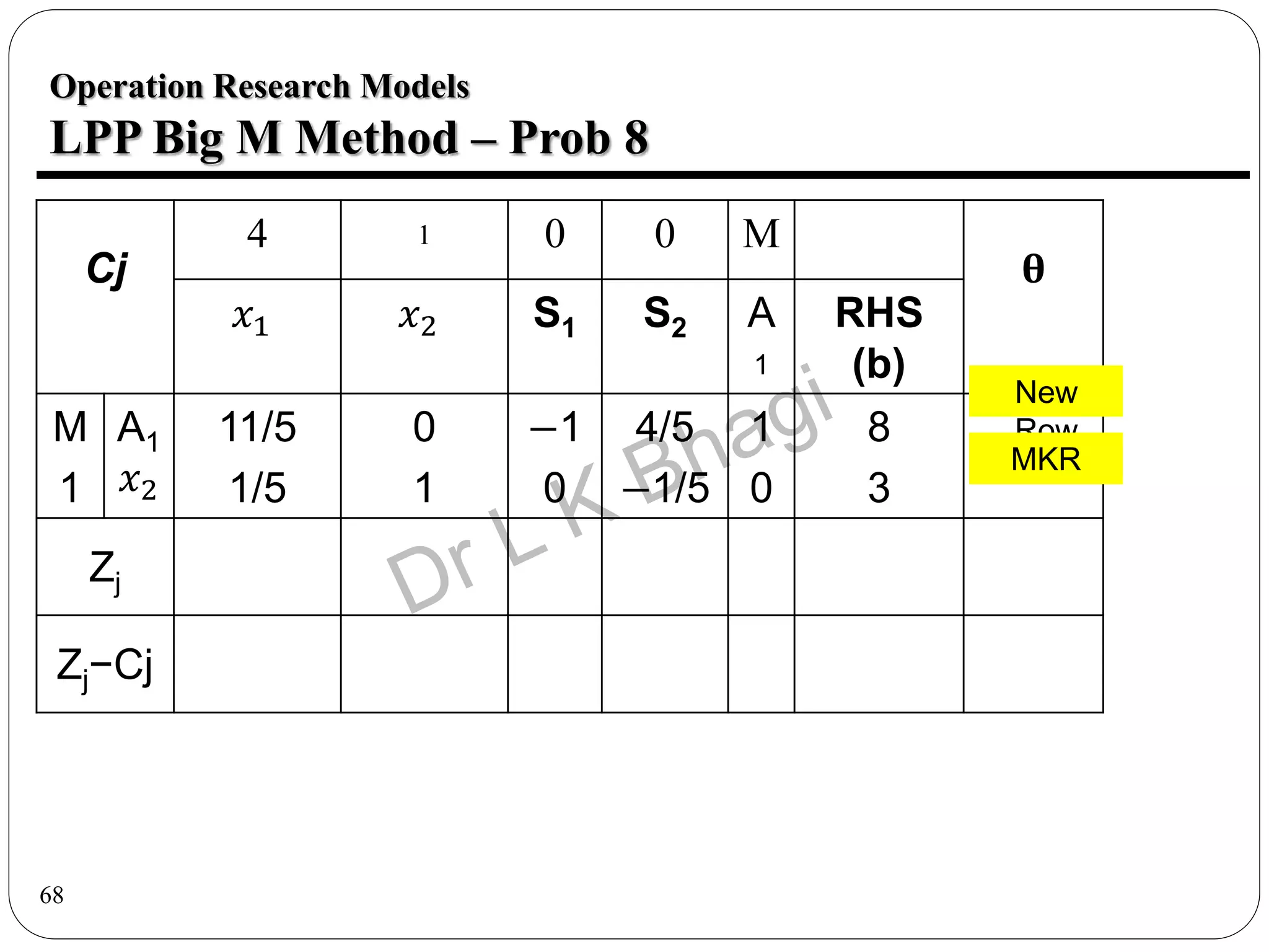
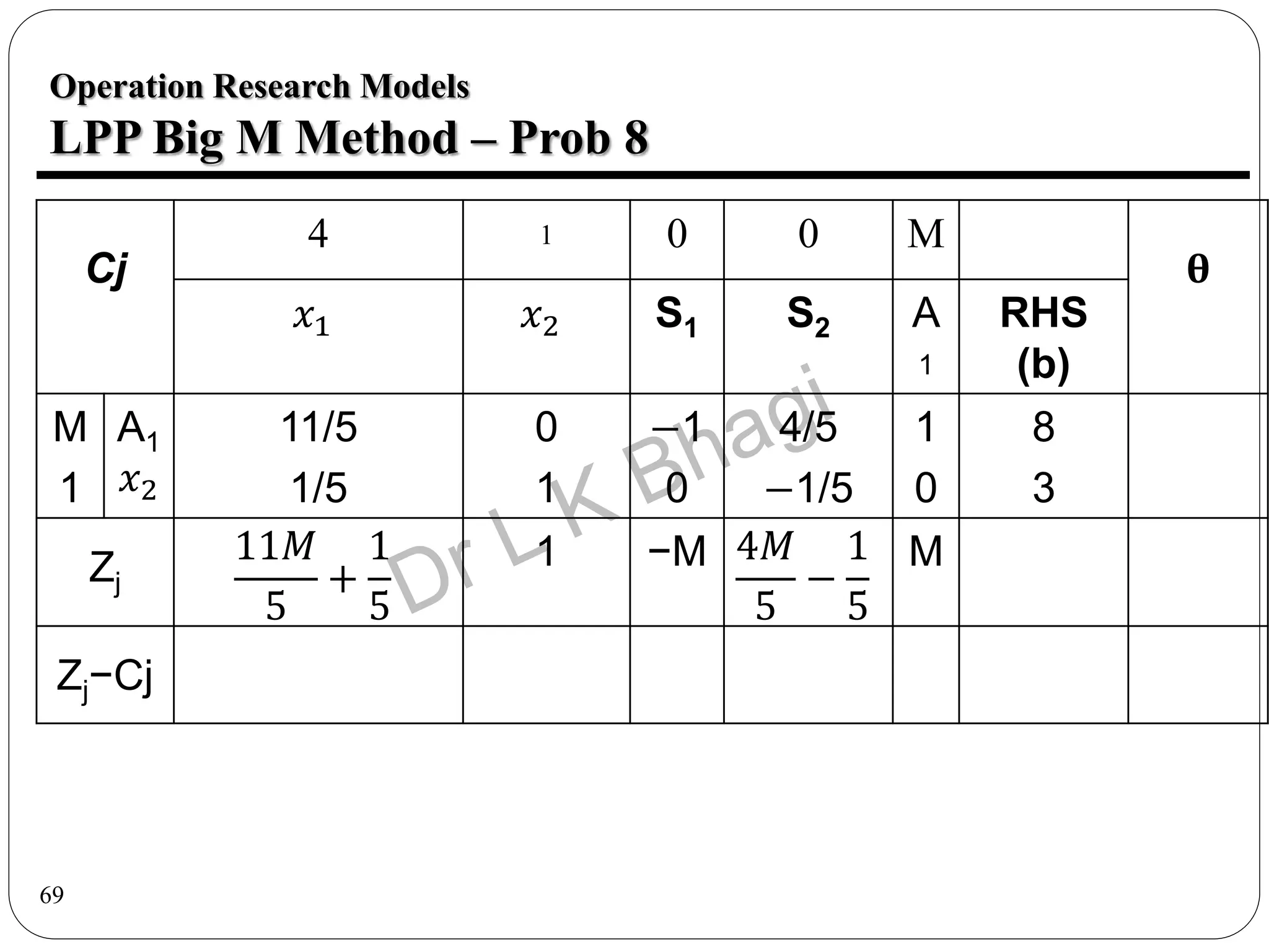
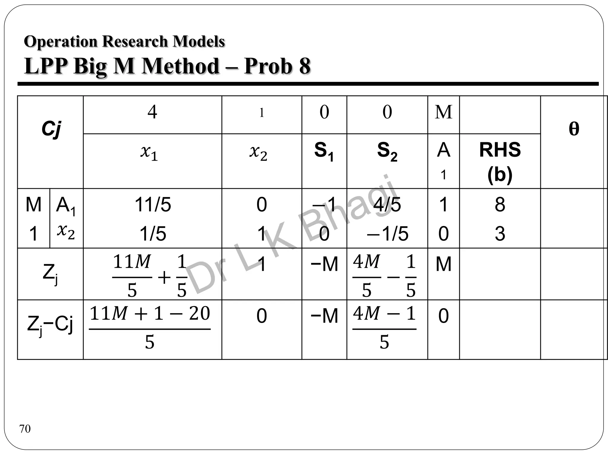
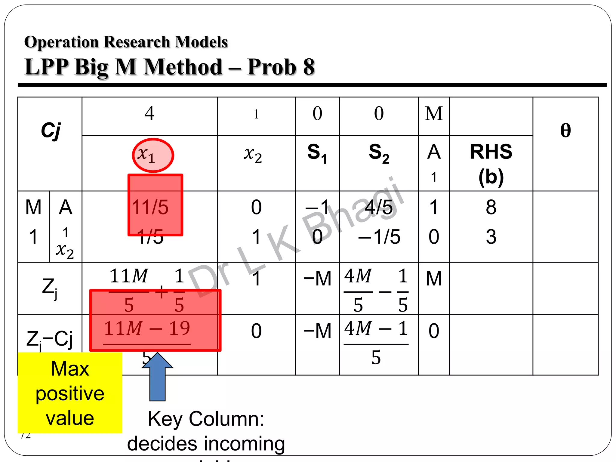
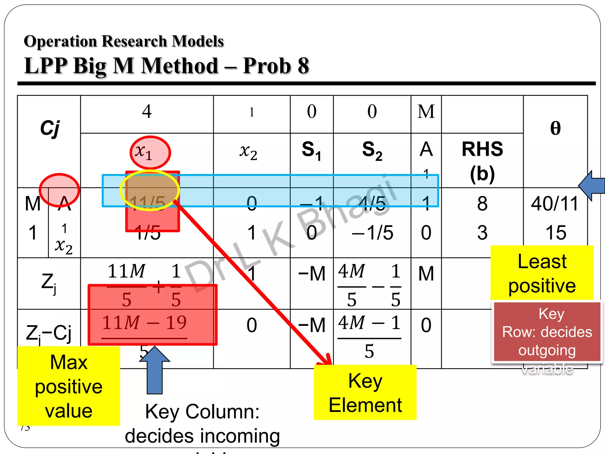
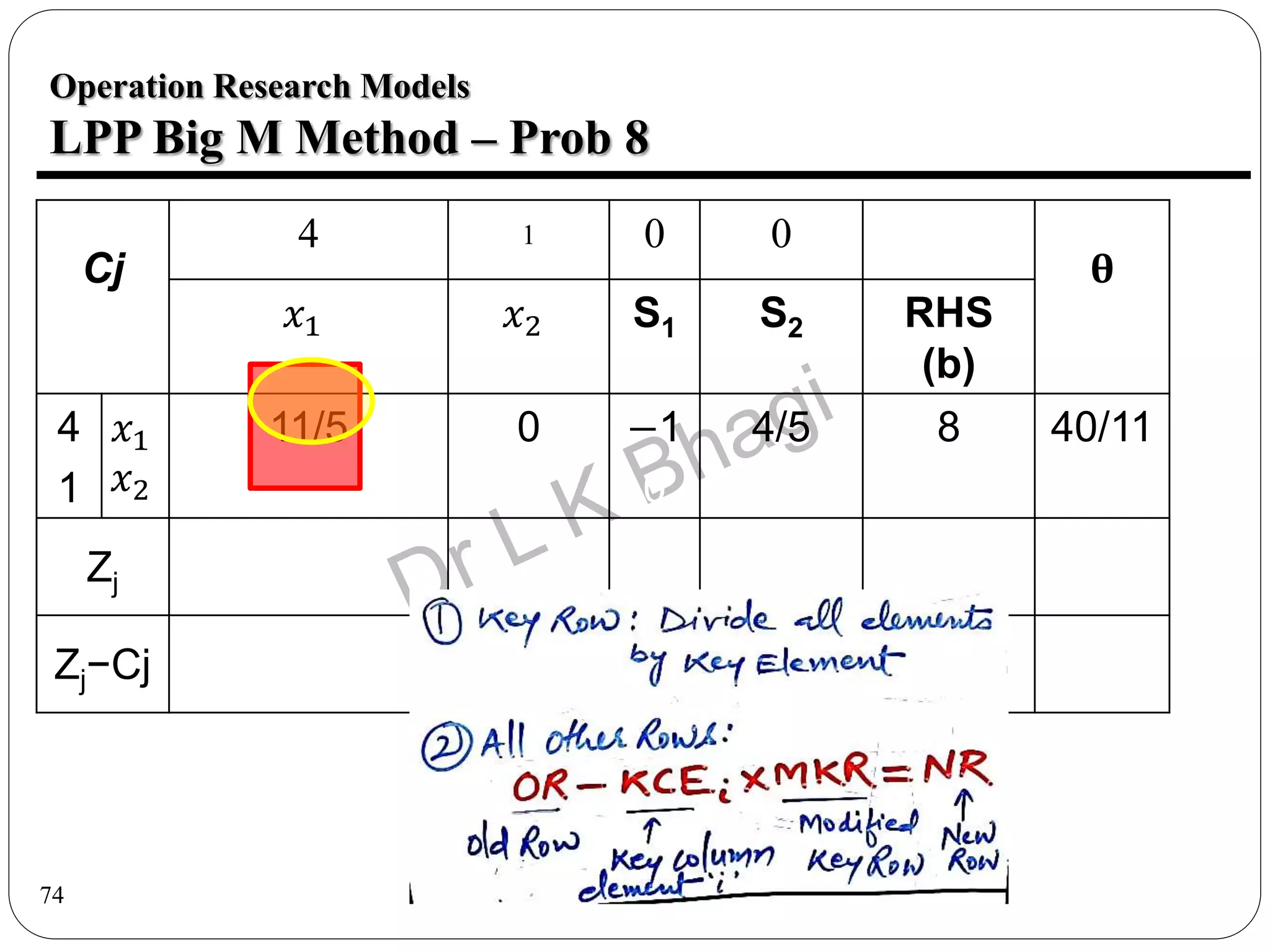
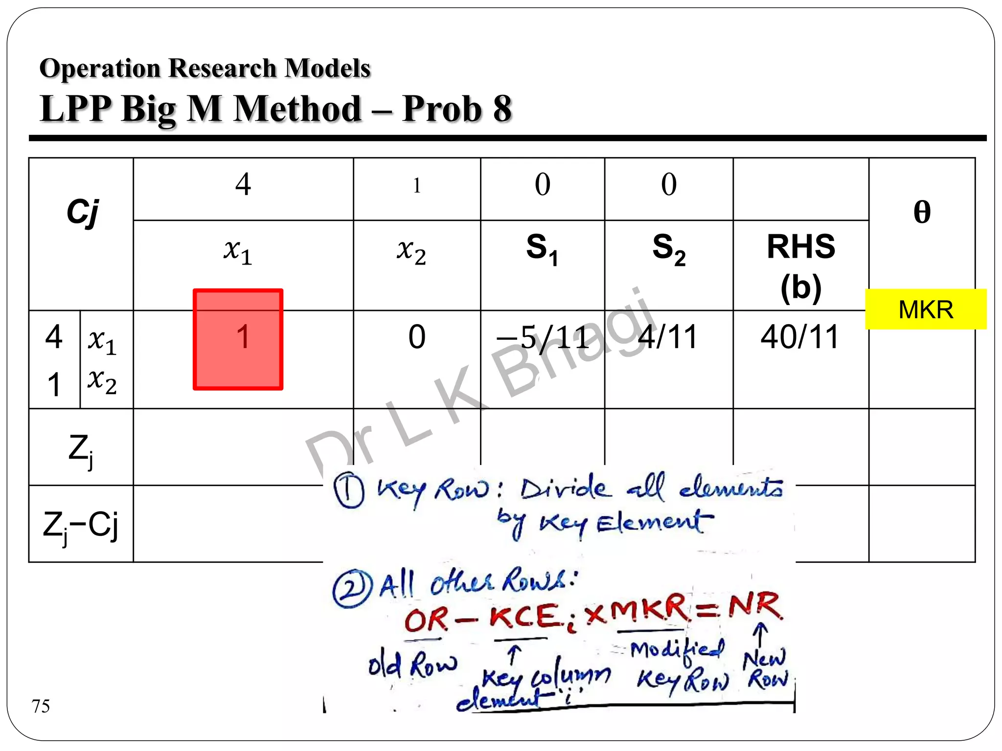
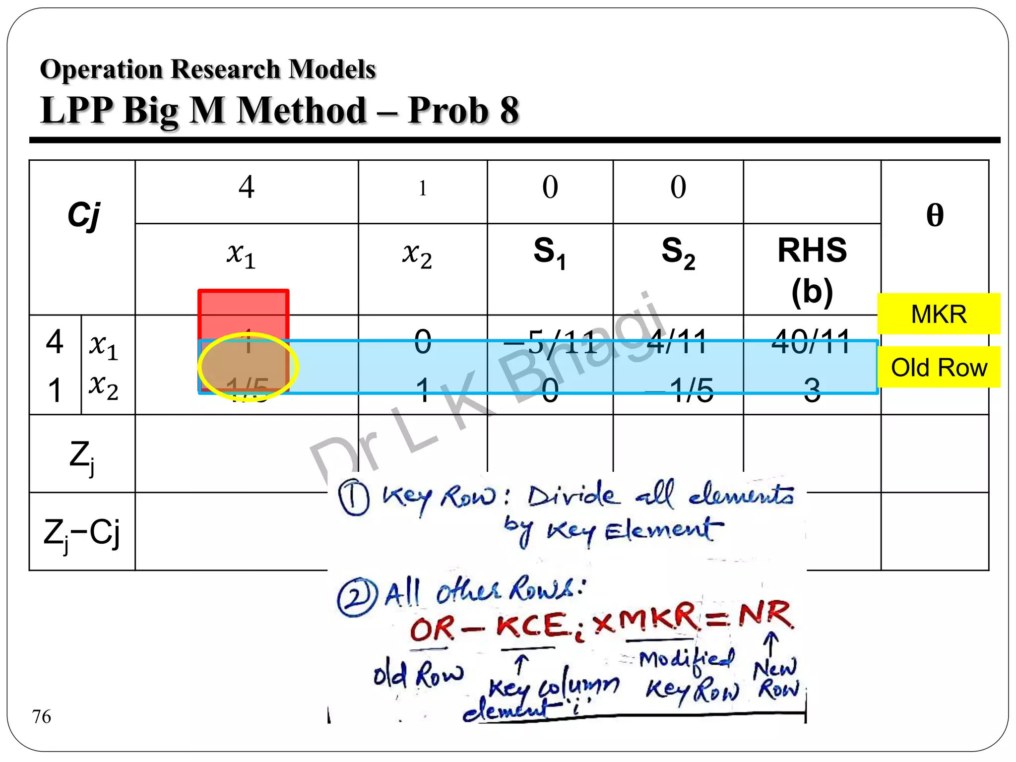
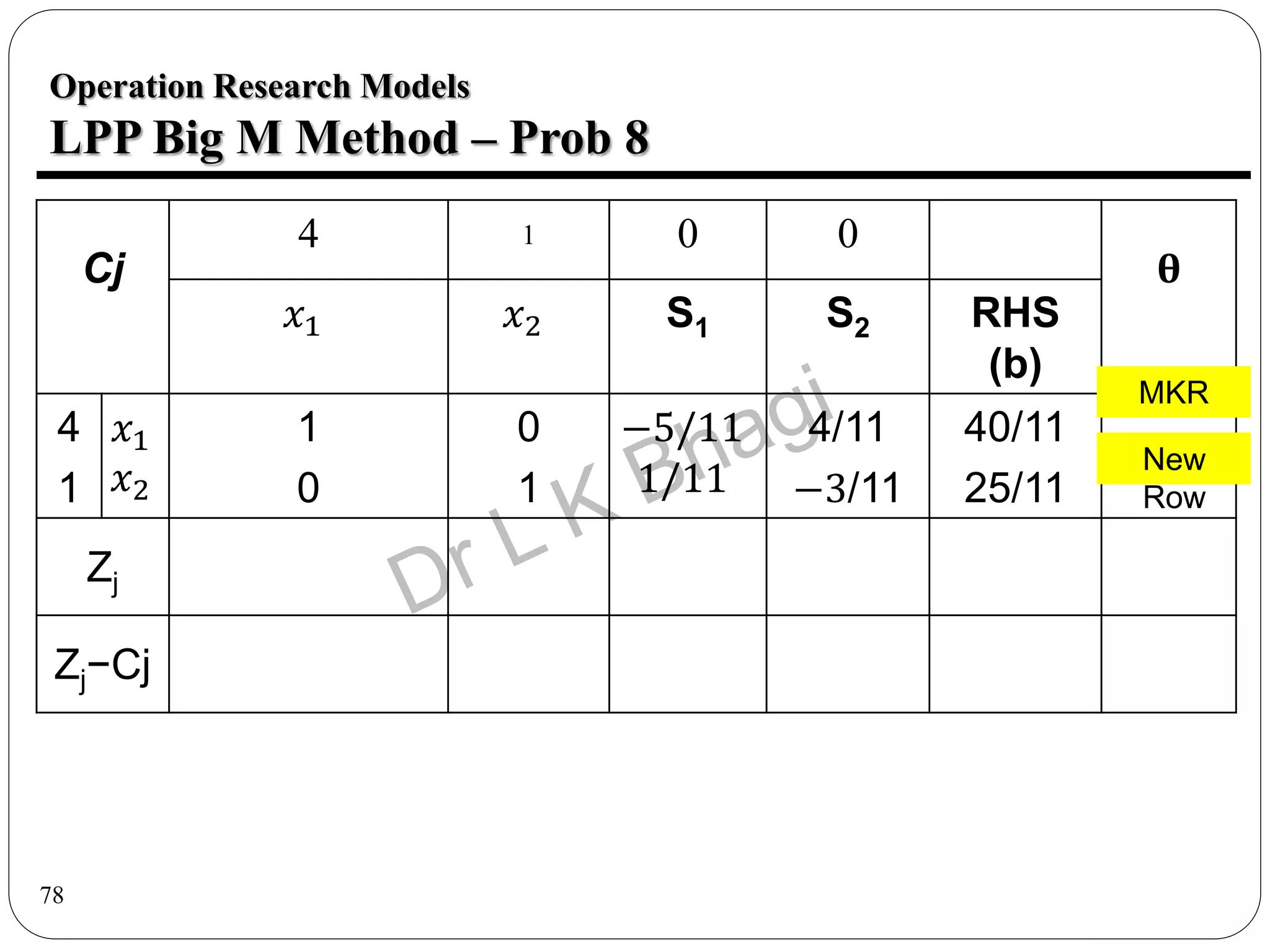
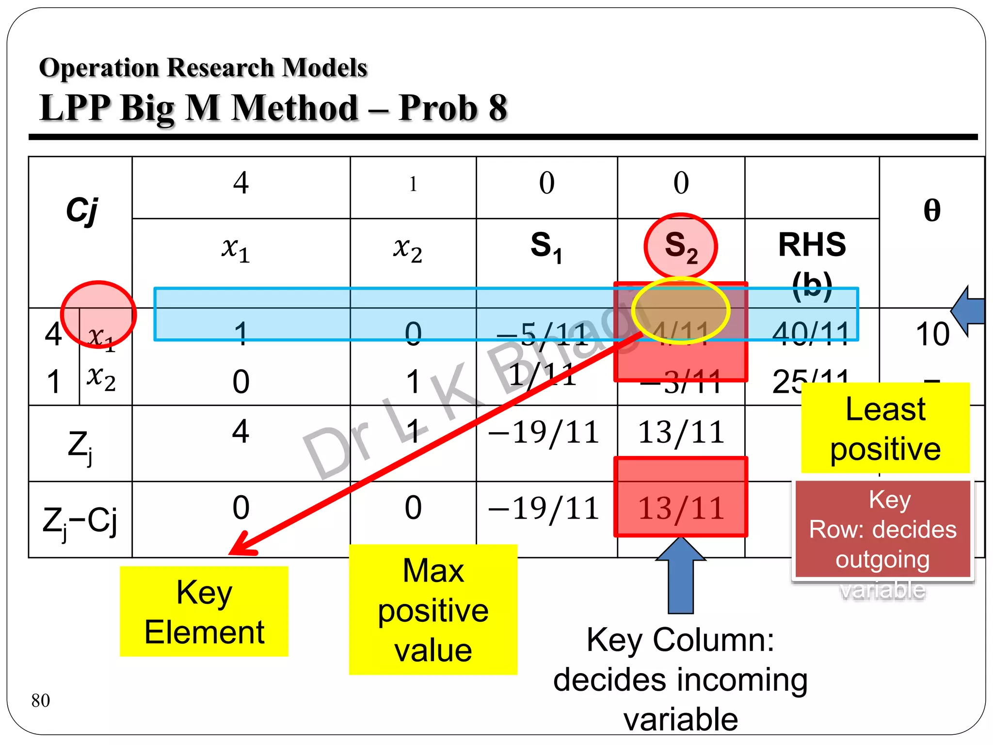
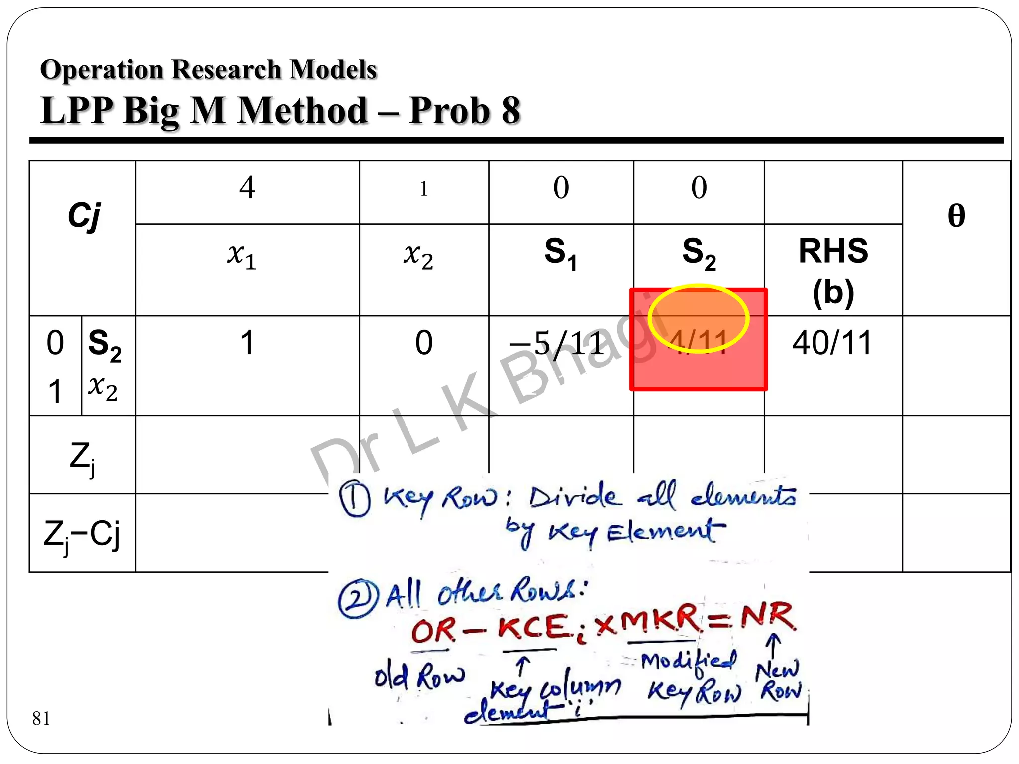
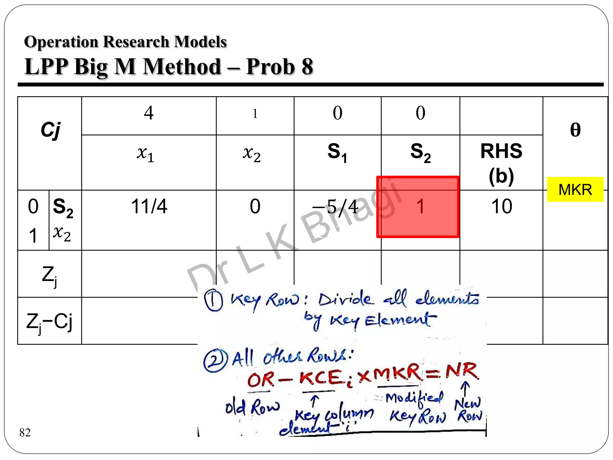
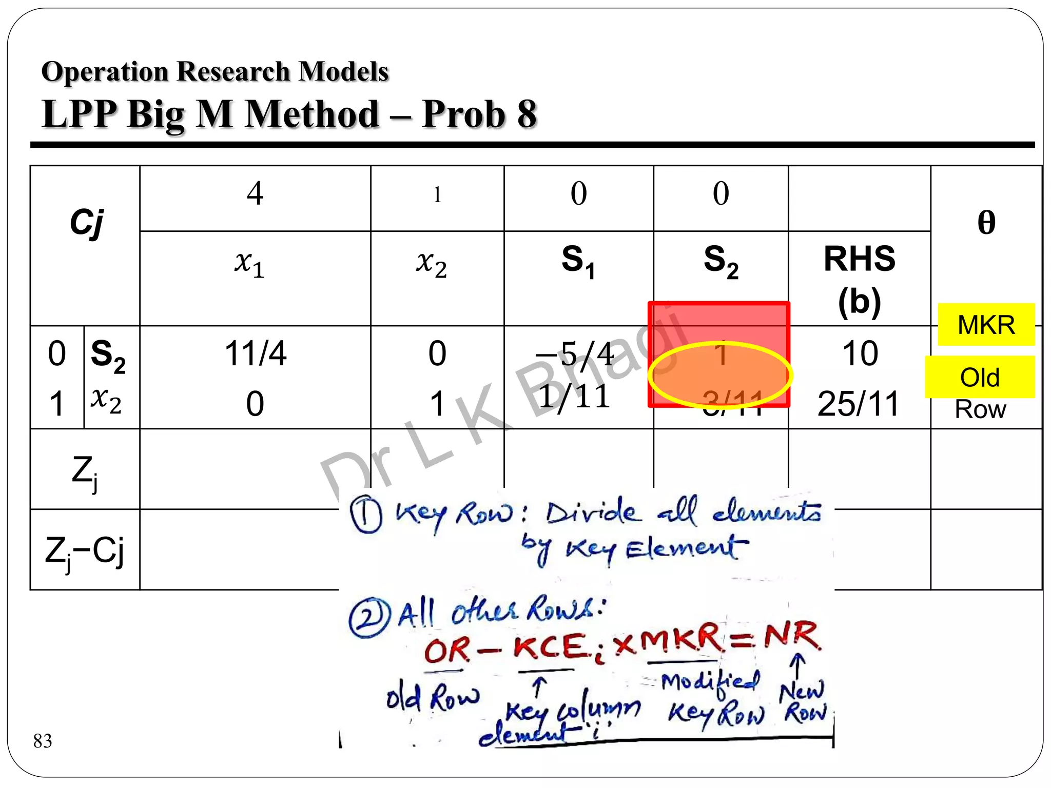
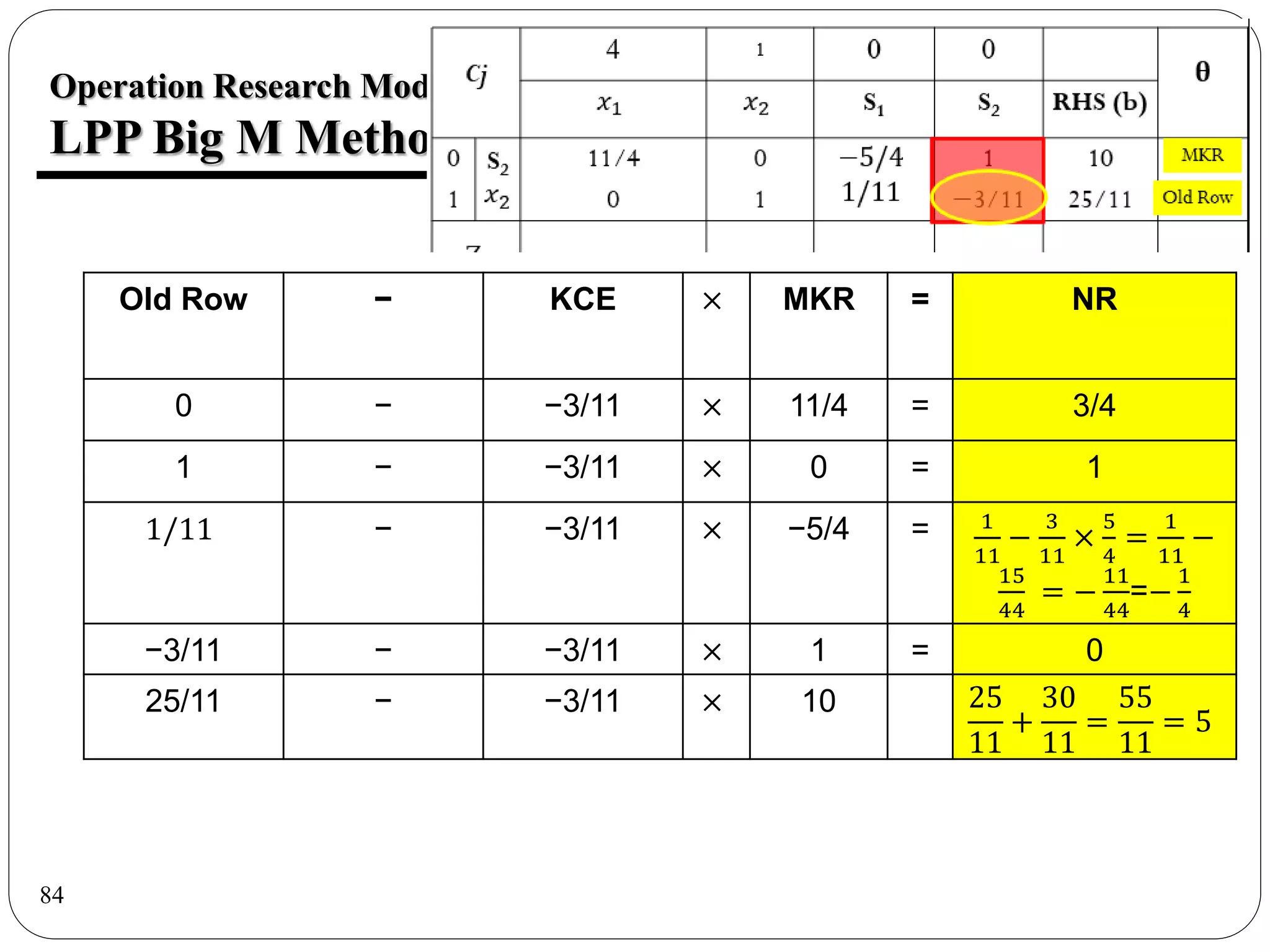
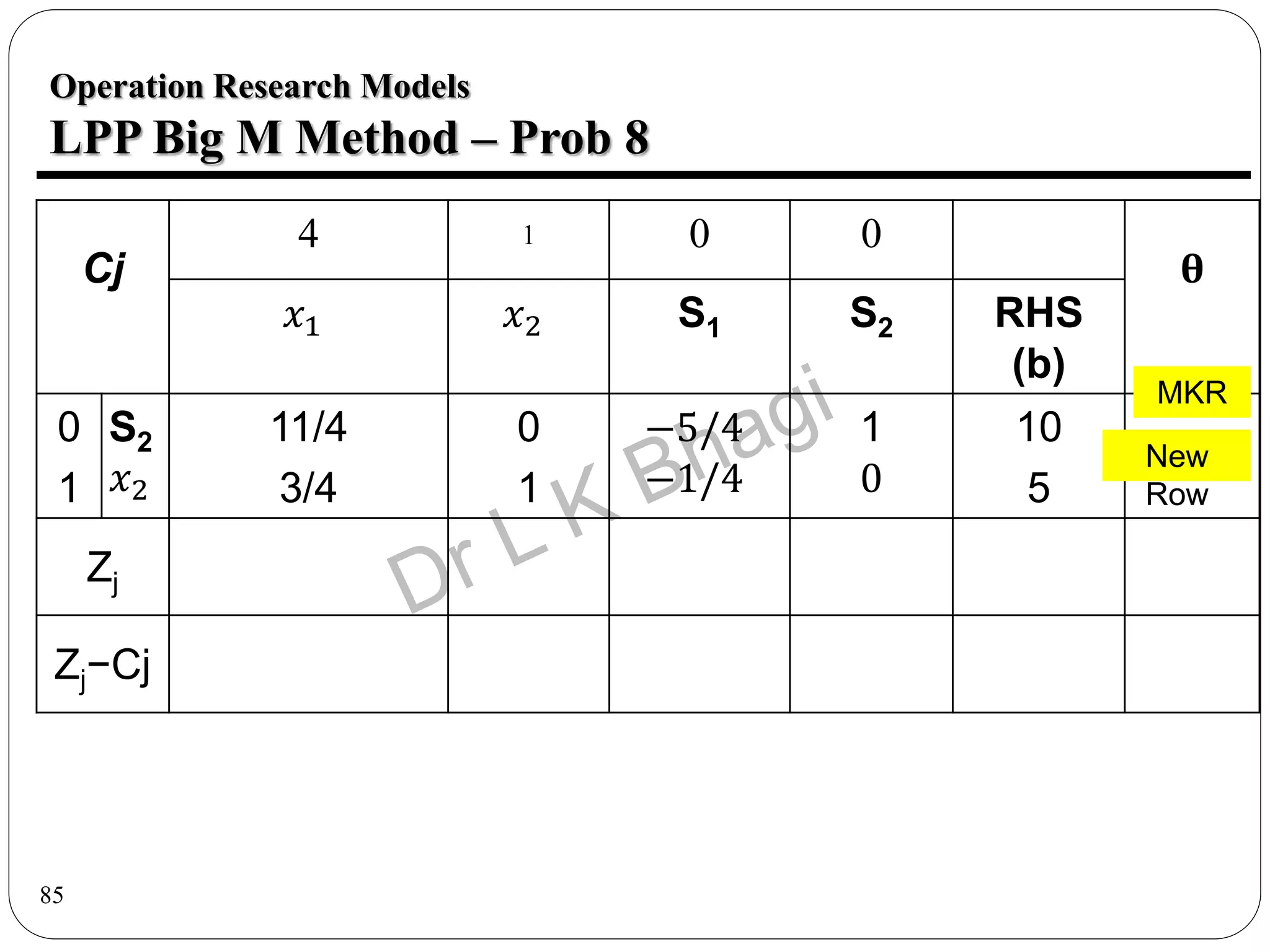
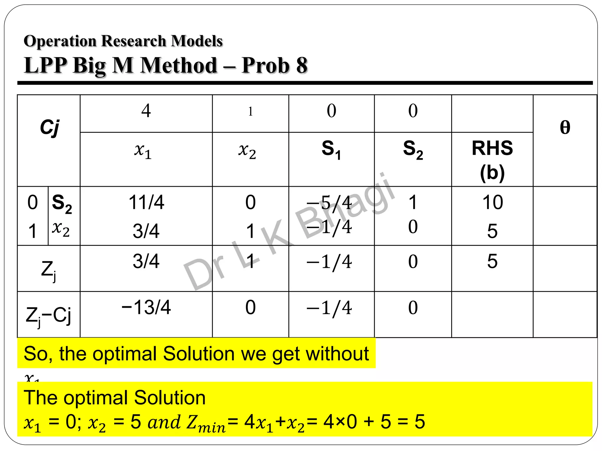
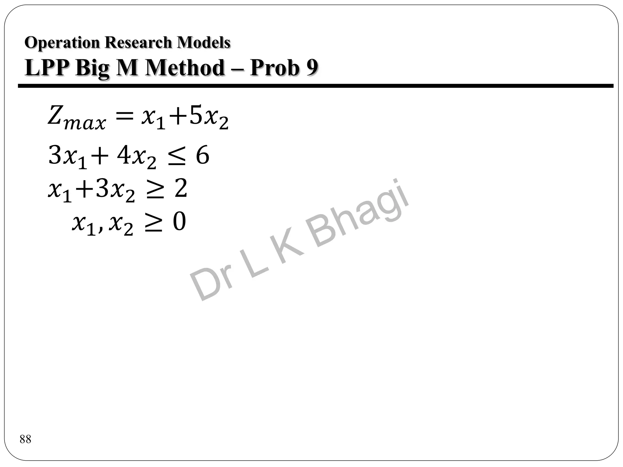
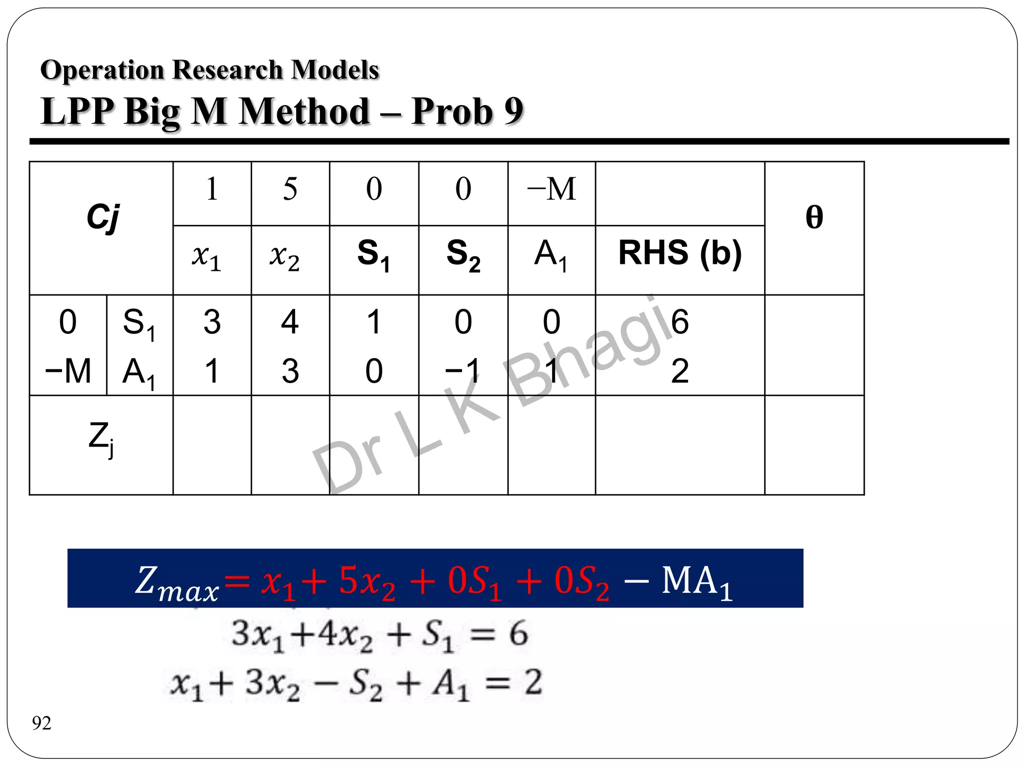
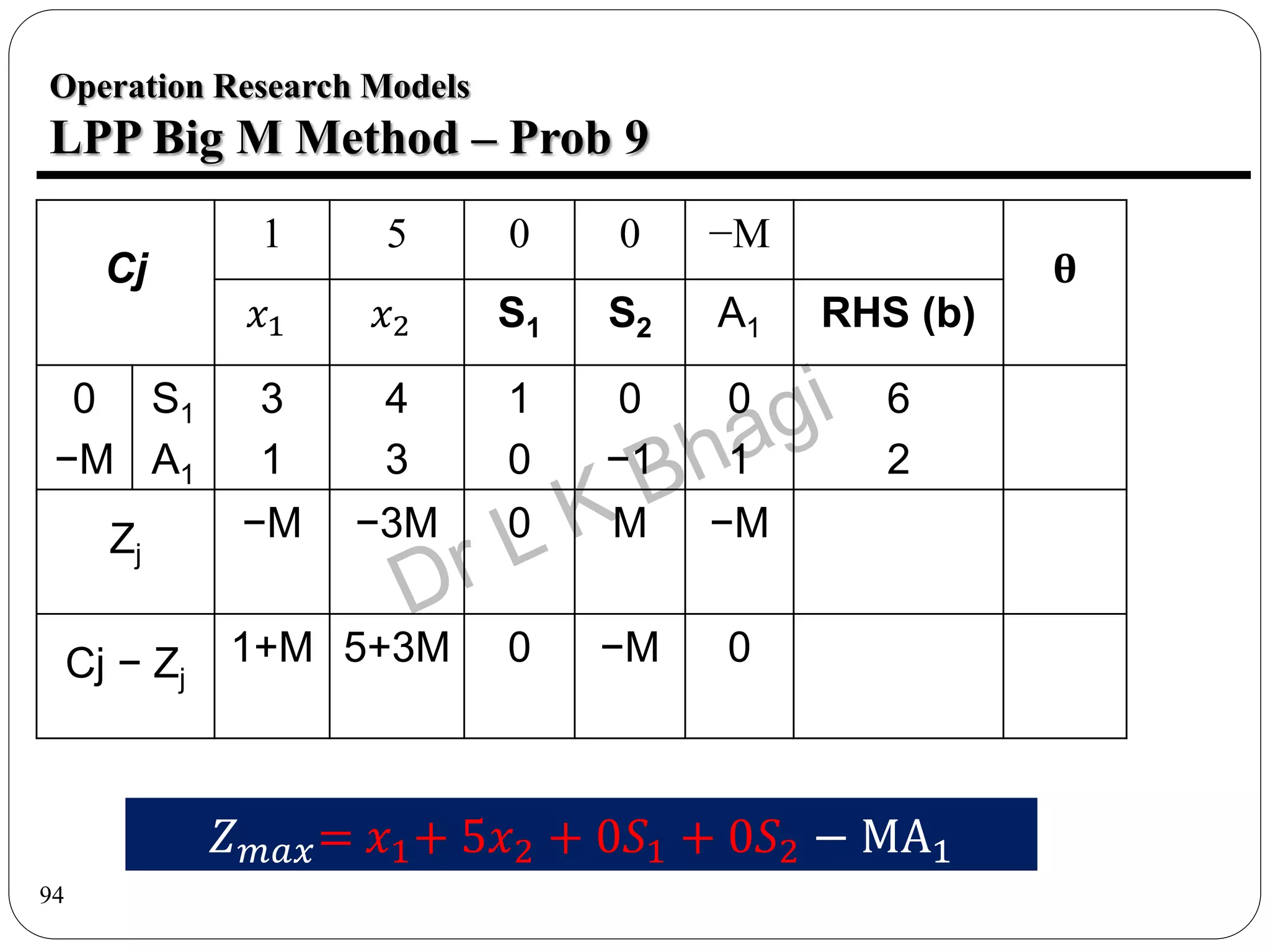
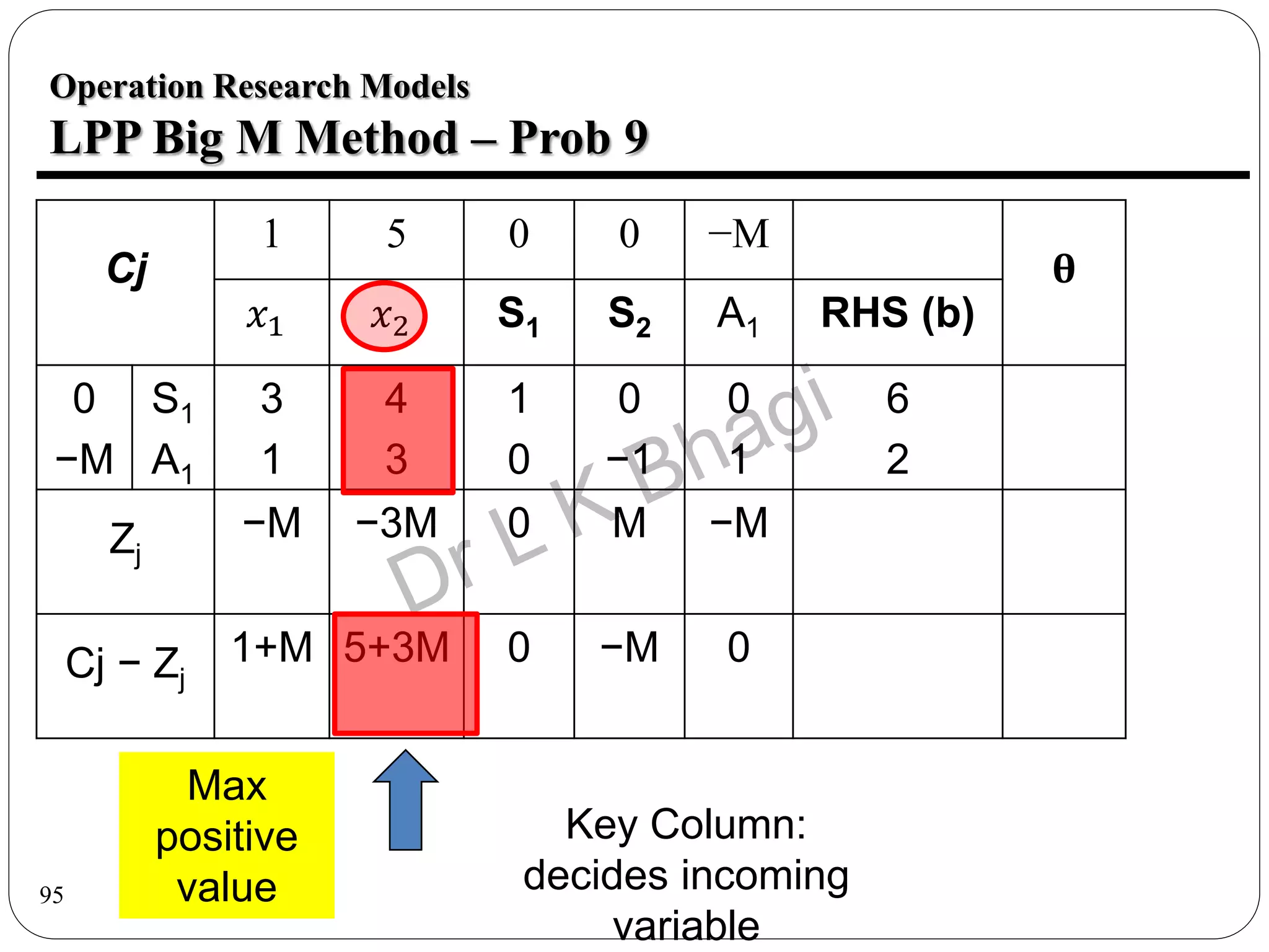
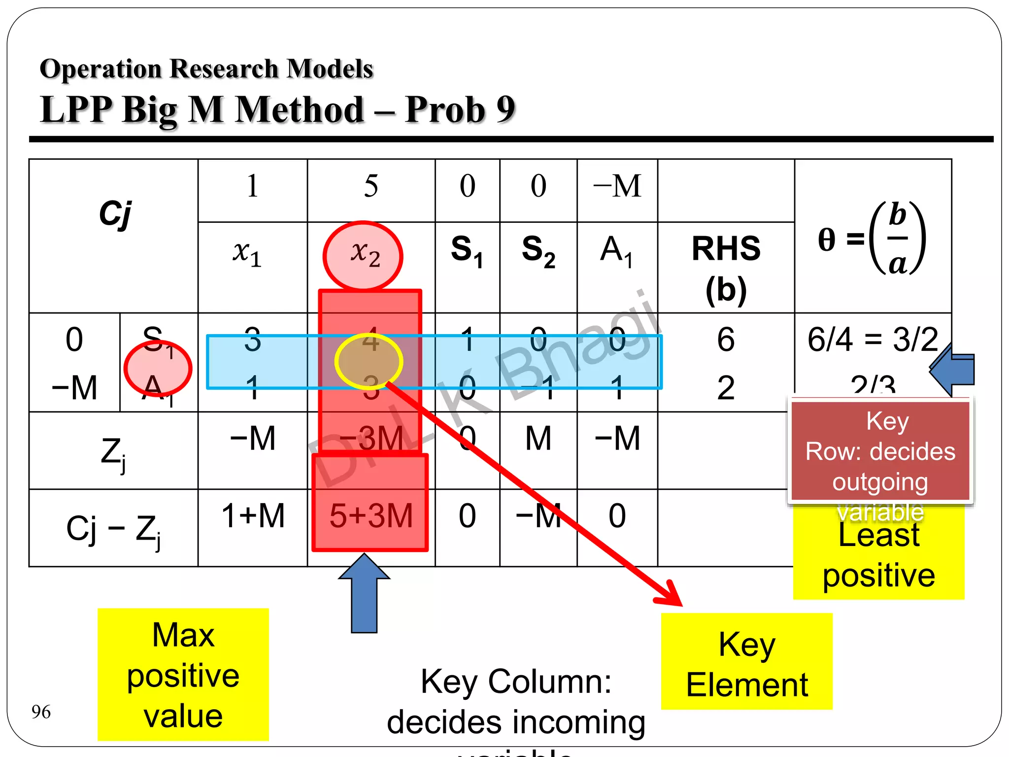
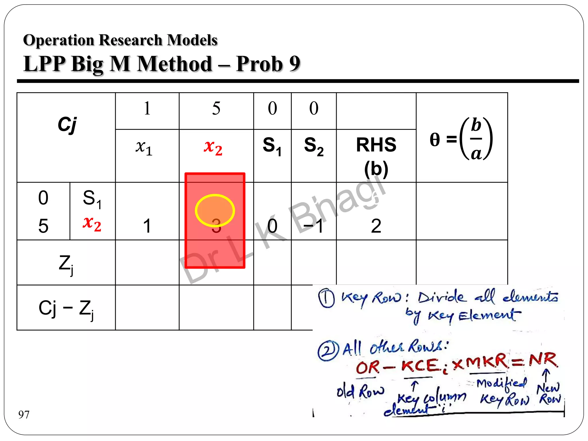
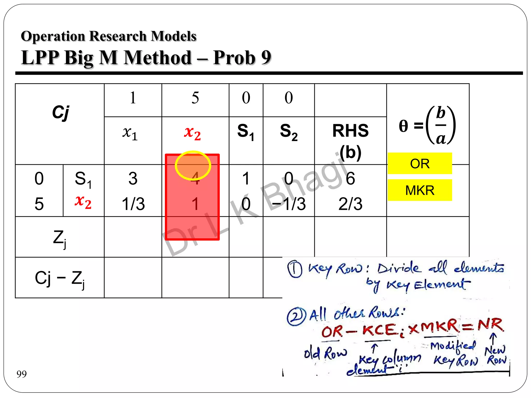
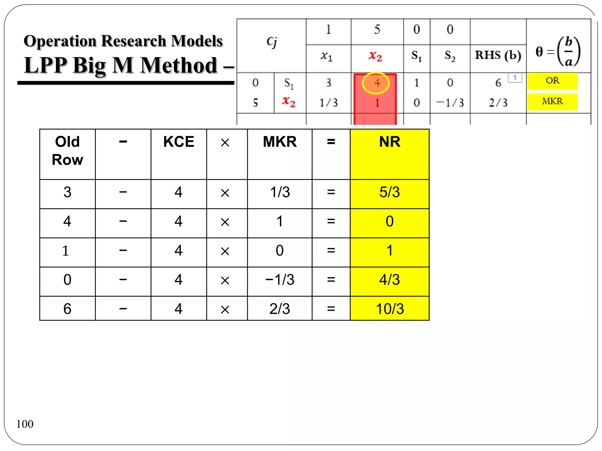
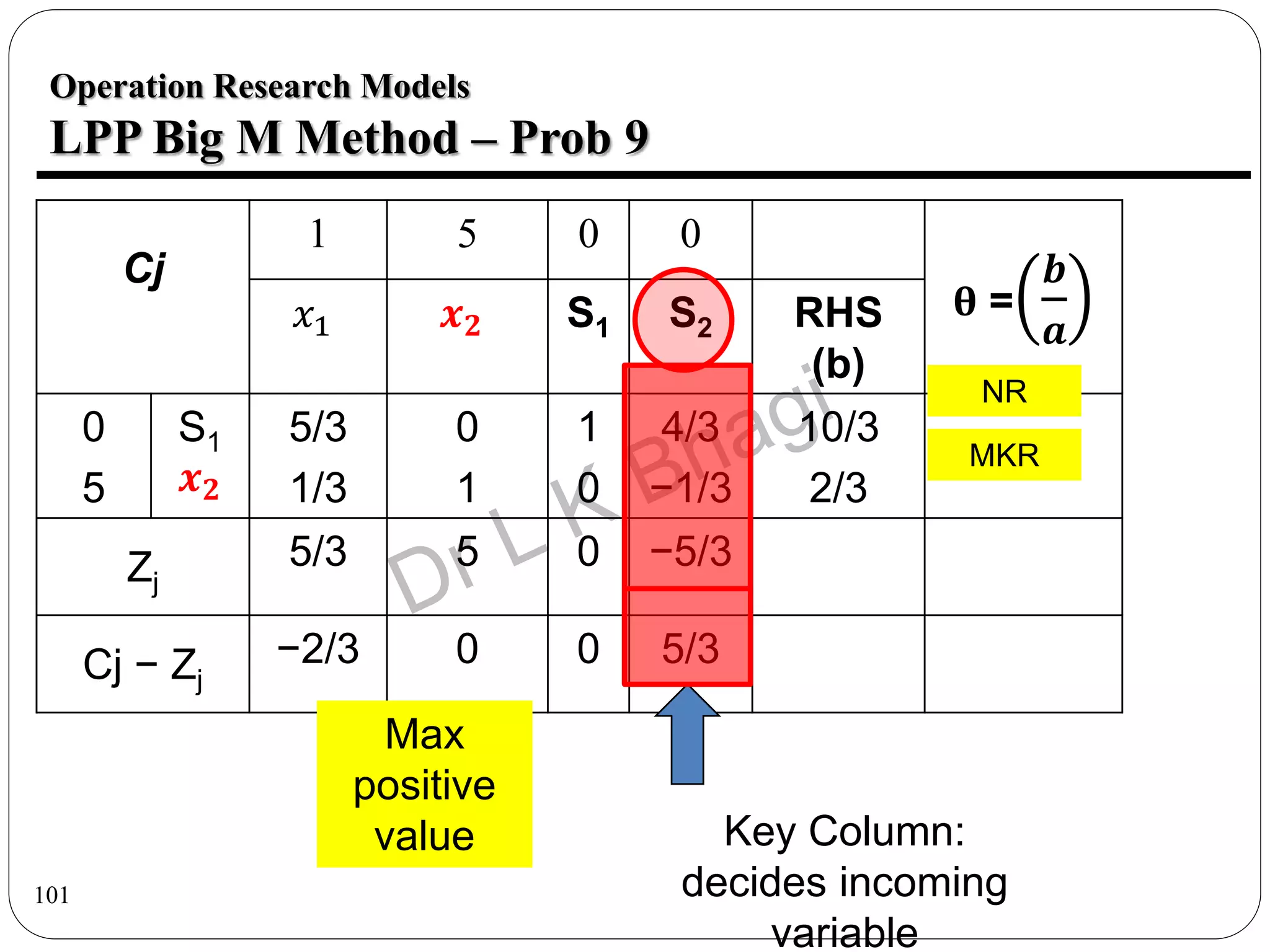
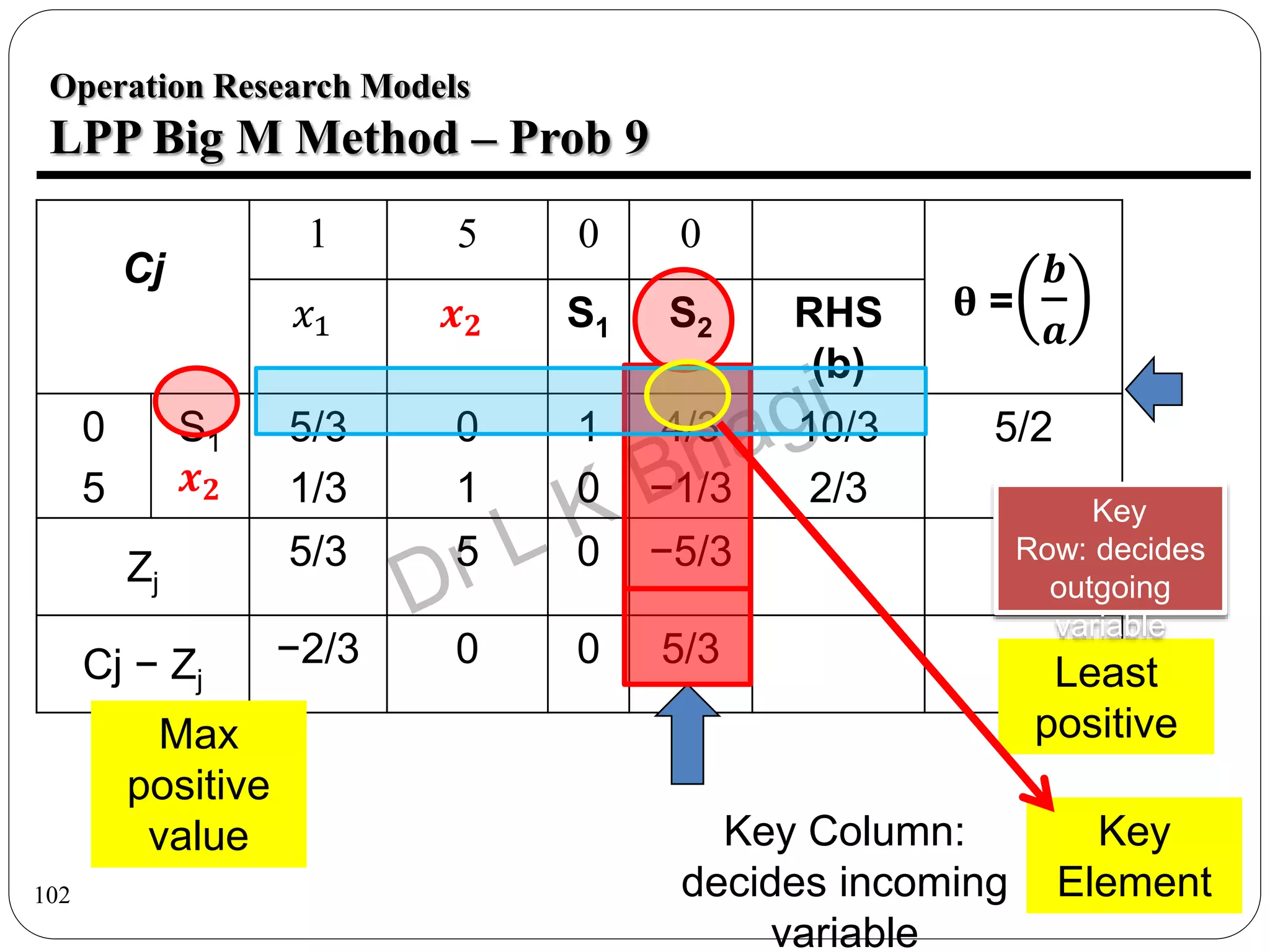
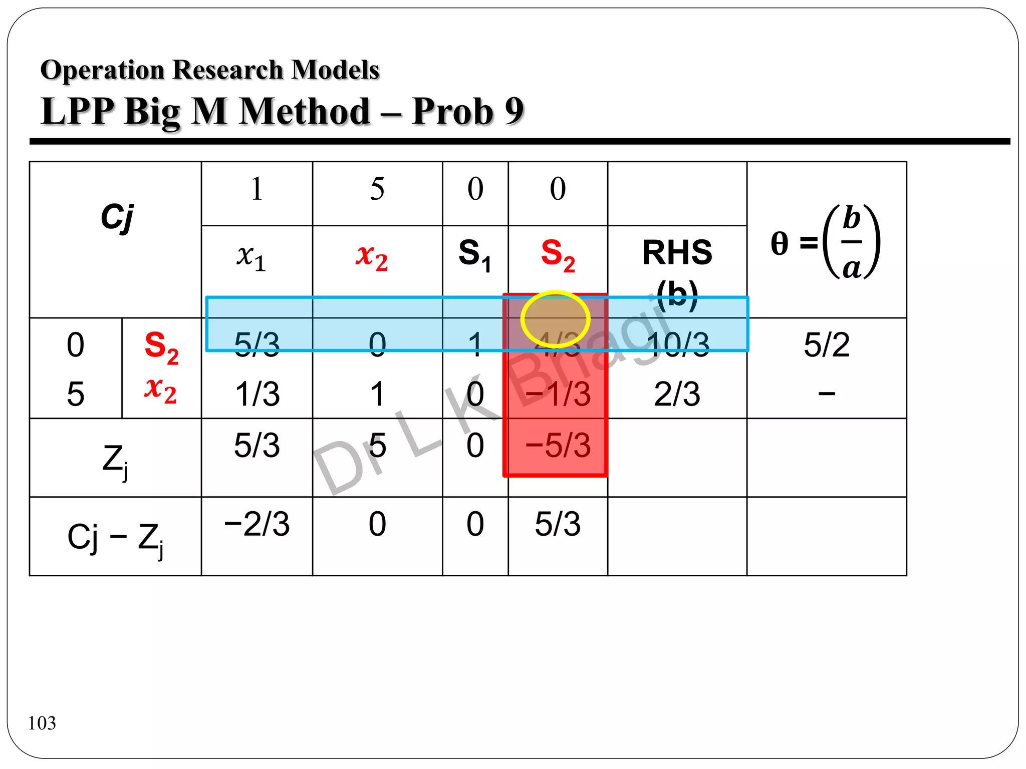
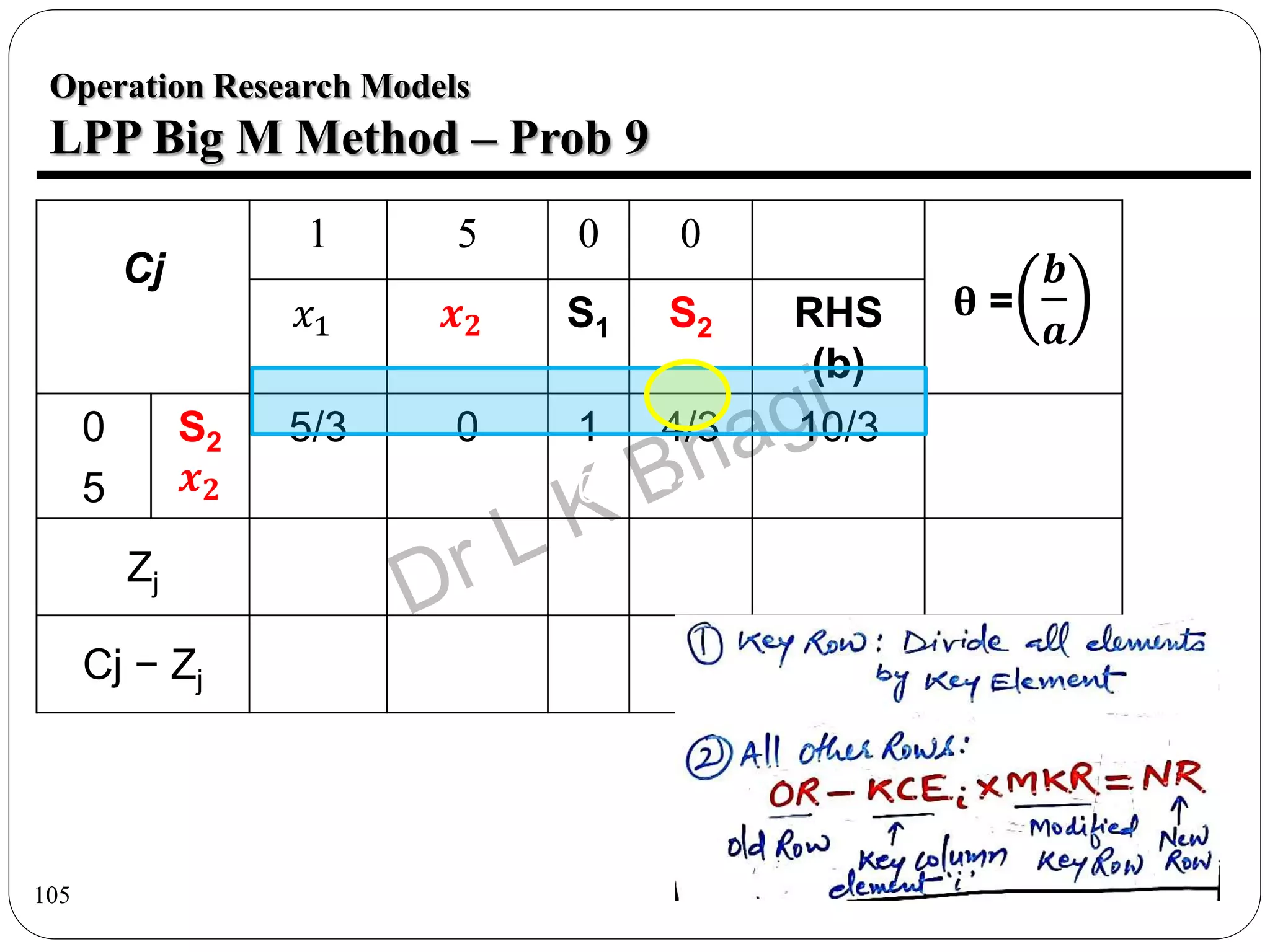
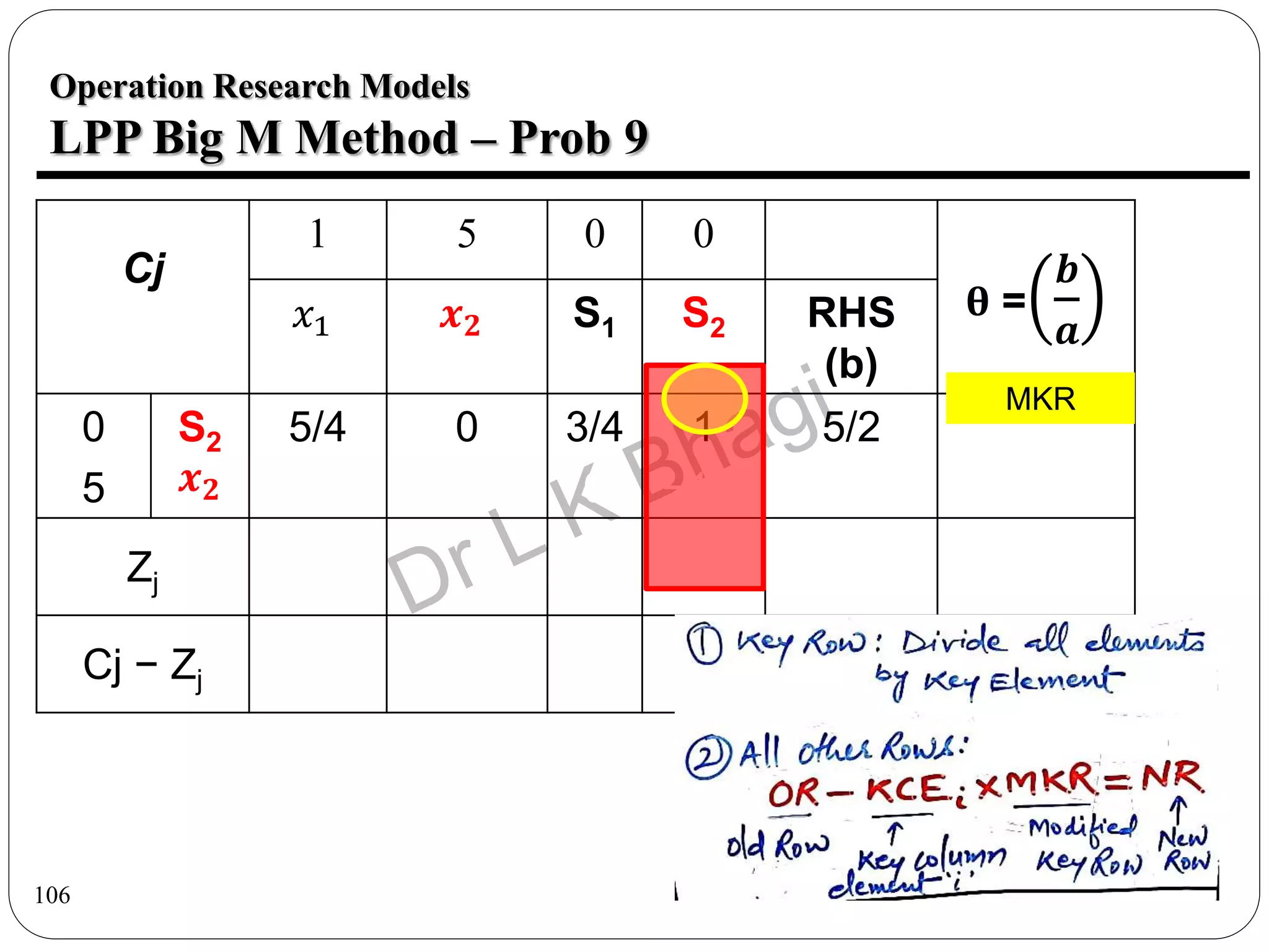
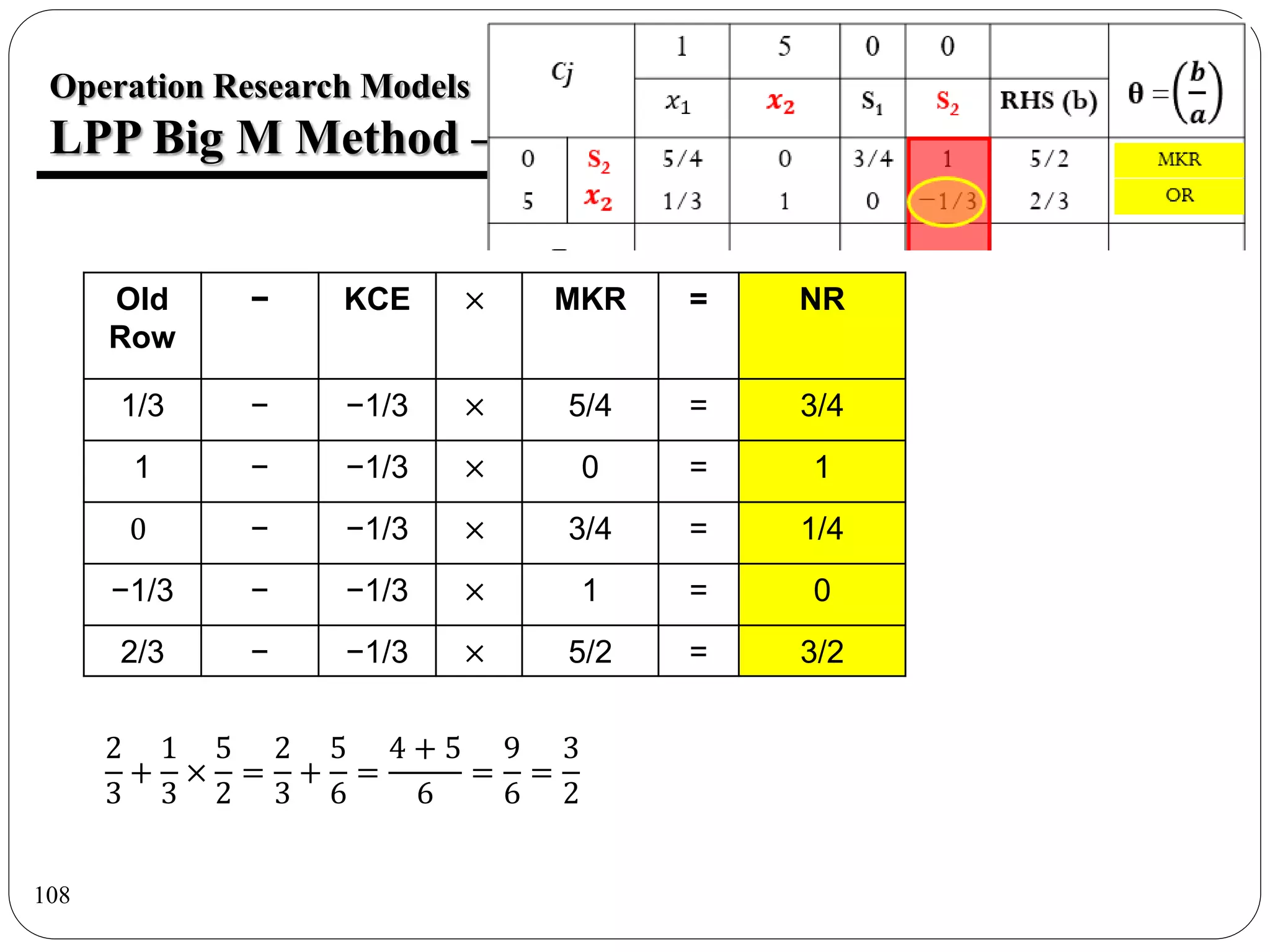
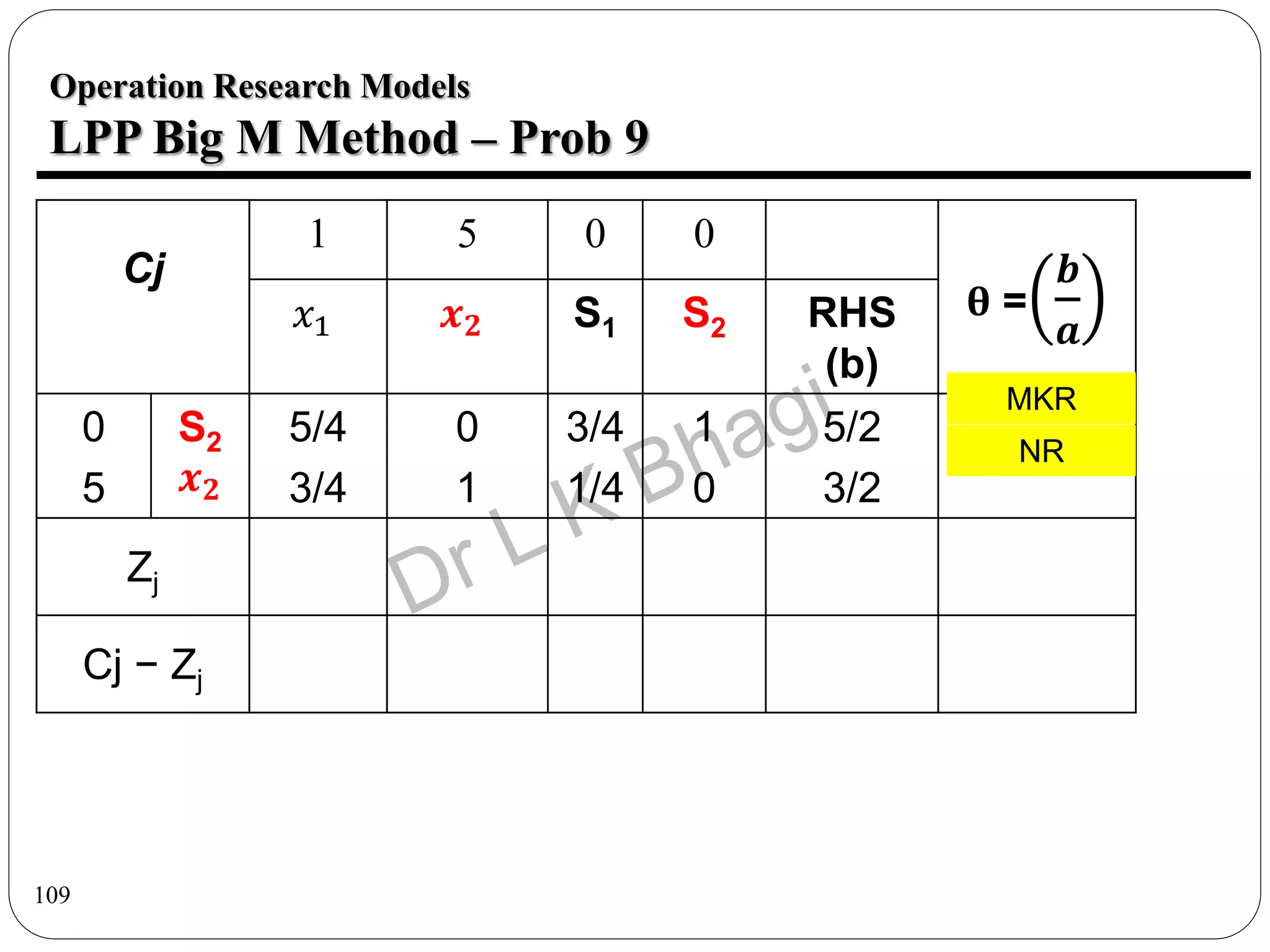
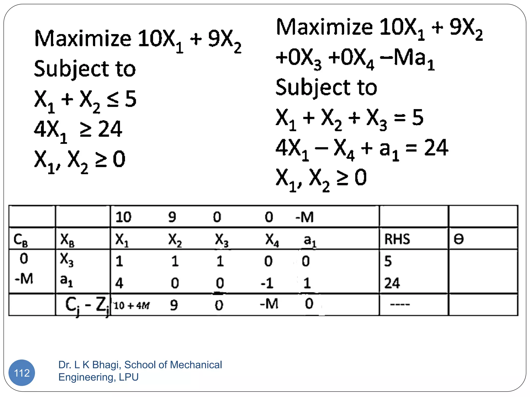
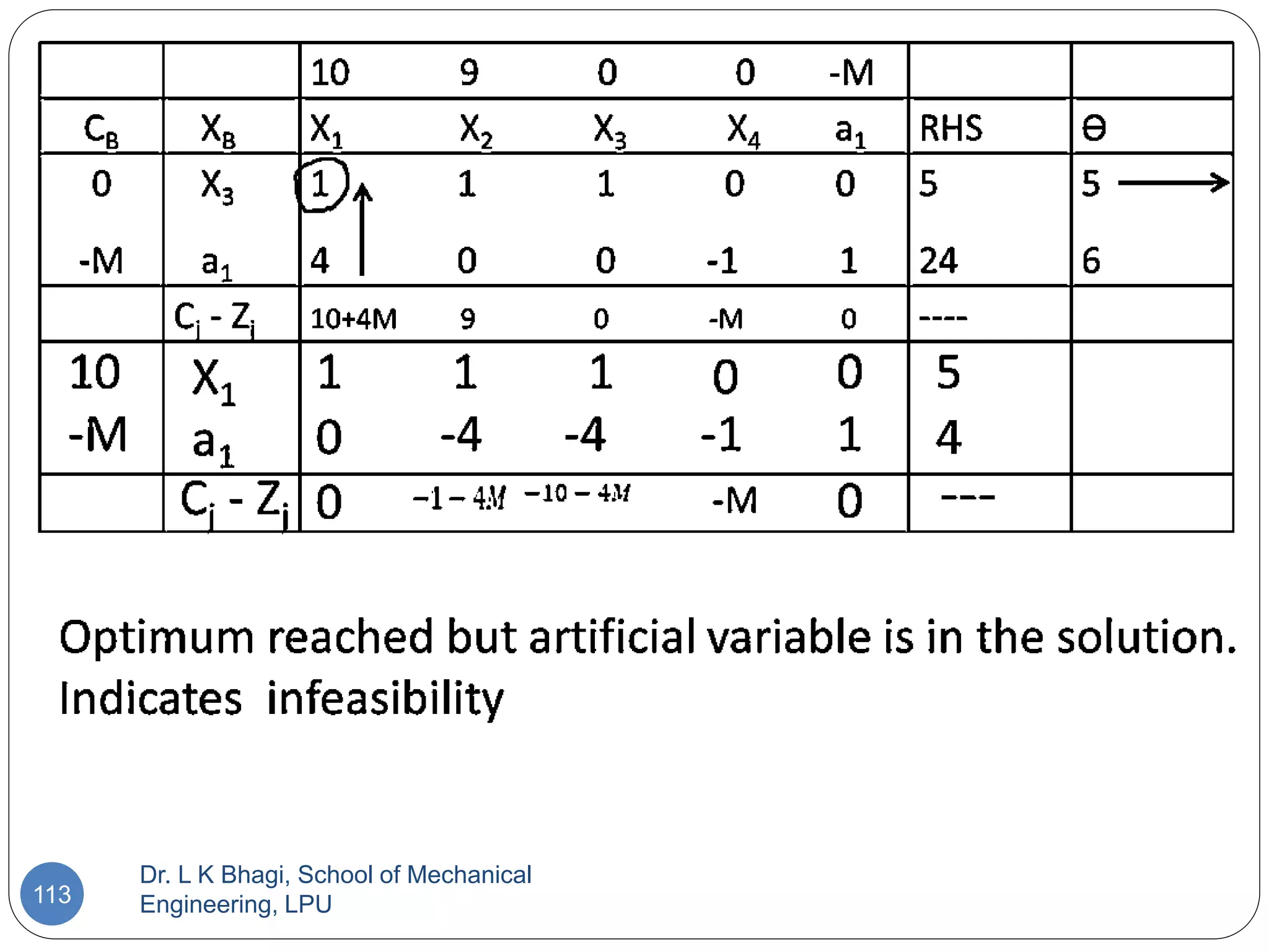
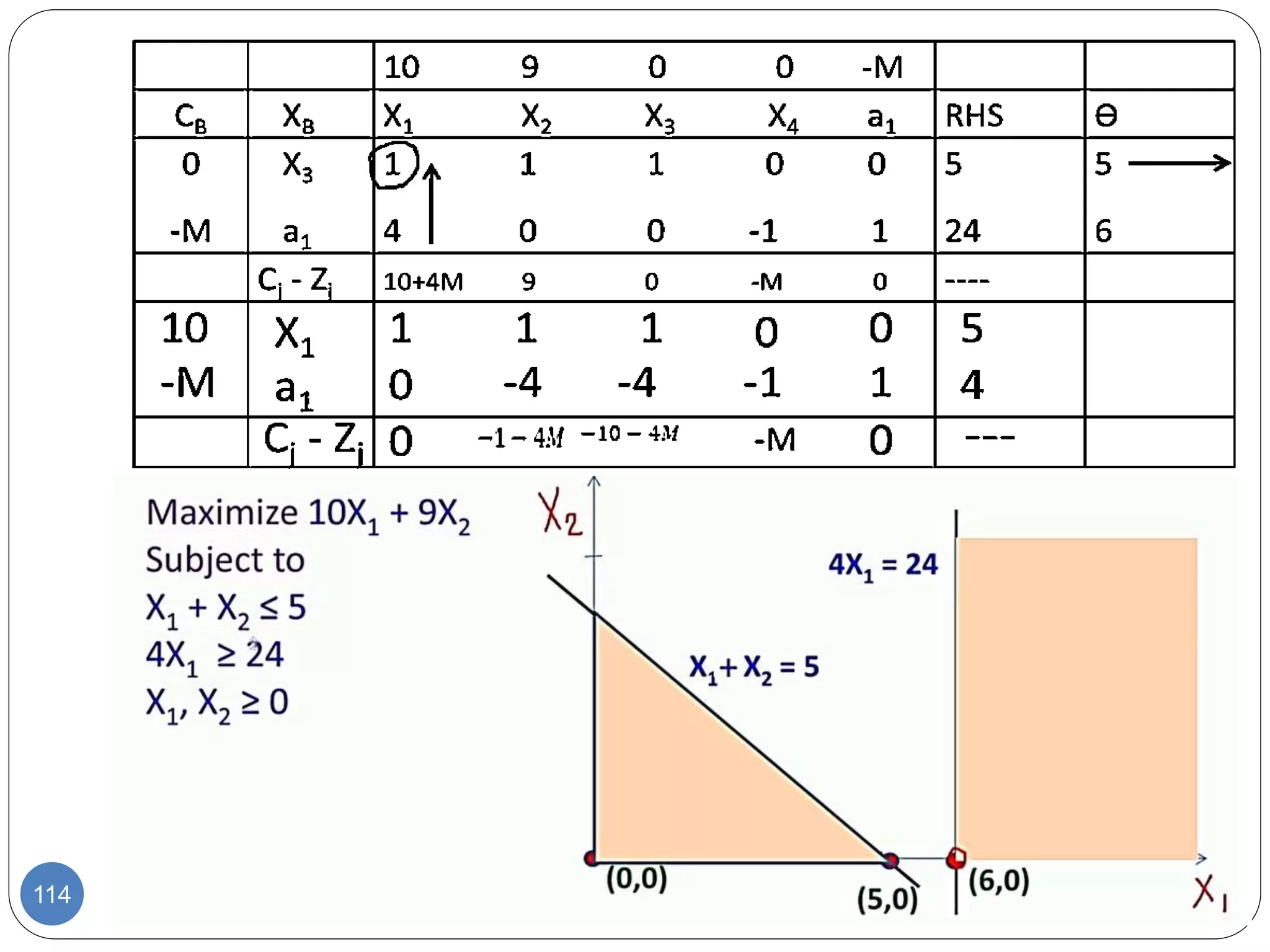
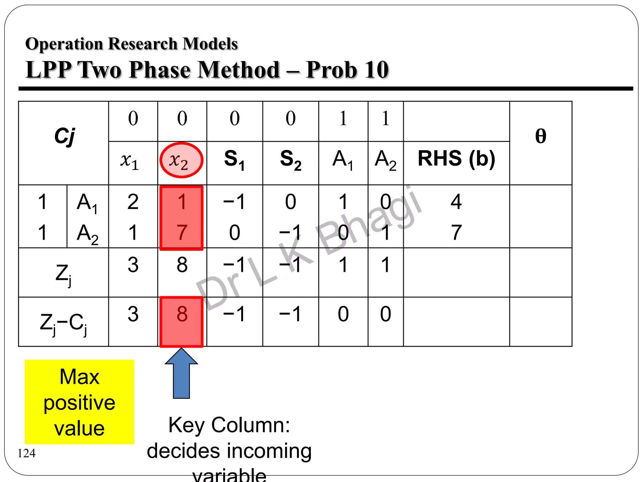
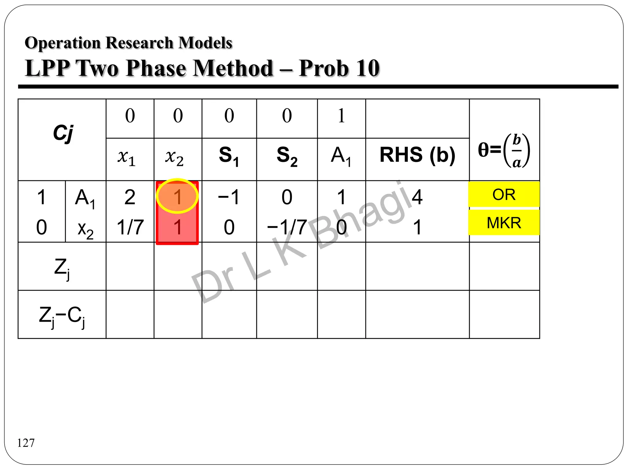
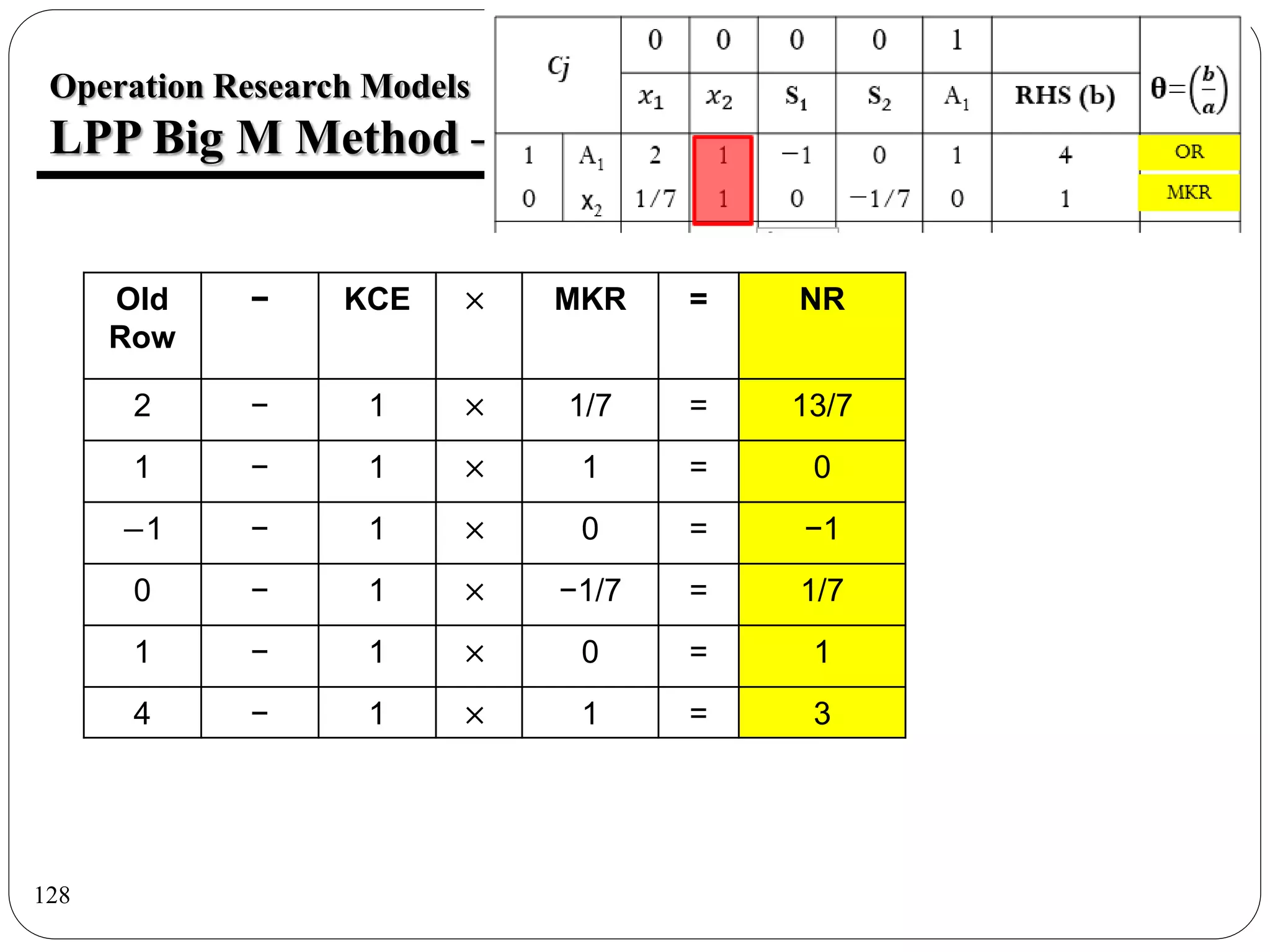
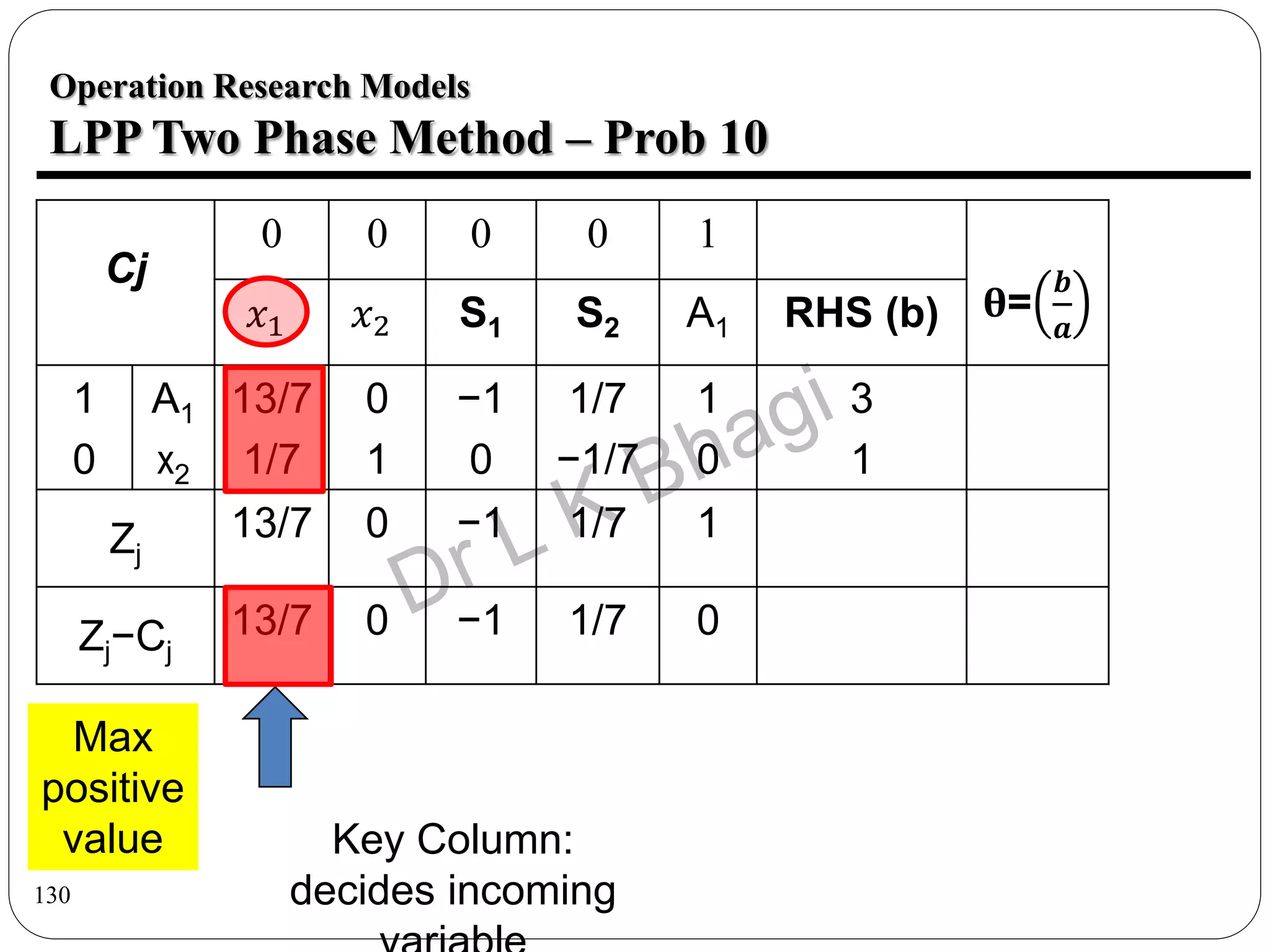
The document discusses the application of the Big M method within linear programming, focusing on formulating constraints as equations by introducing slack, surplus, and artificial variables. It presents multiple examples and step-by-step solutions to demonstrate the method's use in determining optimal solutions. Overall, it serves as a guide for implementing operational research models using the Big M approach.

1. Linear Programming
UNIT – I
OPERATION RESEARCH
Dr. Loveleen Kumar Bhagi
Associate Professor
School of Mechanical Engineering
LPU

2. BIG M Method

3. Dr. L K Bhagi, School of Mechanical
Engineering, LPU
3

4. Dr. L K Bhagi, School of Mechanical
Engineering, LPU
4

5. 5
Operation Research Models
LPP Big M Method
Simplex method Big M method

6. 6
Zmin= 6X+8Y
X+Y ≥ 10
2X +3Y ≥ 25
X +5Y ≥ 35
X, Y ≥ 0
Add slack Surplus
variable to convert
constraint equation into
equality
Z = 6X+8Y+0S1 − 0S2
− 0S3
X+Y−S1 =10
2X +3Y−S2 = 25
X +5Y − S3 = 35
X,Y, S1, S2, S3 ≥ 0
Operation Research Models
LPP Big M Method – Prob 7

7. 7
Ibfs (Initial Basic Feasible Solution)
DV = 0
−S =10 ; −S2 = 25; − S3 = 35 0r
S = − 10 ; S2 = − 25; S3 = − 35 0r
Z = 6X+8Y+0S1 − 0S2 − 0S3
X+Y−S1 =10
2X +3Y−S2 = 25
X +5Y − S3 = 35
X,Y, S1, S2, S3 ≥ 0
Operation Research Models
LPP Big M Method – Prob 7

8. 8
Ibfs (Initial Basic Feasible Solution)
DV = 0 and Surplus = 0
0 =10 ; 0 = 25; 0 = 35
Z = 6X+8Y+0S1 − 0S2 − 0S3
X+Y−S1 =10
2X +3Y−S2 = 25
X +5Y − S3 = 35
X,Y, S1, S2, S3 ≥ 0
Operation Research Models
LPP Big M Method – Prob 7

9. 9
X+Y ≥ 10
2X +3Y ≥ 25
X +5Y ≥ 35
X, Y ≥ 0
Along with Surplus
variable add Artificial
Variable to convert
constraint equation into
equality
X+Y−S1 +A1 =10
2X +3Y−S2+A2 = 25
X +5Y − S3 +A3 = 35
X,Y, S1, S2, S3, A1, A2, A3
≥ 0
Operation Research Models
LPP Big M Method – Prob 7
Zmin =
6X+8Y+0S1+0S2+ 0S3+MA1+MA2+MA3
Zmin=
6X+8Y

10. 10
Operation Research Models
LPP Big M Method – Prob 7
Zmin =
6X+8Y+0S1+0S2+ 0S3+MA1+MA2+MA3
Ibfs (Initial Basic Feasible Solution)
Put DV = 0 and Surplus variables = 0
A1=10 ;
A2= 25;
A3= 35

11. 11
Operation Research Models
LPP Big M Method – Prob 7
Cj
6 8 0 0 0 M M M
θ
X Y S1 S2 S3 A1 A2 A3 RHS
(b)
M
M
M
A1
A2
A3
10
25
35

12. 12
Operation Research Models
LPP Big M Method – Prob 7
Cj
6 8 0 0 0 M M M
θ
X Y S1 S2 S3 A1 A2 A3 RHS
(b)
M
M
M
A1
A2
A3
1
2
1
1
3
5
−1
0
0
0
−1
0
0
0
−1
1
0
0
0
1
0
0
0
1
10
25
35

13. 13
Operation Research Models
LPP Big M Method – Prob 7
Cj
6 8 0 0 0 M M M
θ
X Y S1 S2 S3 A
1
A
2
A3 RHS
(b)
M
M
M
A1
A2
A3
1
2
1
1
3
5
−1
0
0
0
−1
0
0
0
−1
1
0
0
0
1
0
0
0
1
10
25
35
Zj
4
M
9
M
−M −M −M M M M
M+2M+M = 4M

14. Dr. L K Bhagi, School of Mechanical
Engineering, LPU
14
https://www.youtube.com/watch?v=tRNwz
Sr9IXg
IITM Srinivasan sir

15. 15
Operation Research Models
LPP Big M Method – Prob 7
Cj
6 8 0 0 0 M M M
θ
X Y S1 S2 S3 A
1
A
2
A3 RHS
(b)
M
M
M
A1
A2
A3
1
2
1
1
3
5
−1
0
0
0
−1
0
0
0
−1
1
0
0
0
1
0
0
0
1
10
25
35
10
25/3
7
Zj 4M 9M −M −M −M M M M
Zj− Cj 4M−
6
9M−
8
−M −M −M 0 0 0
Largest
positive
value Key Column:
decides incoming
Least
positive
Key
Row: decides
outgoing
variable

16. 16
Operation Research Models
LPP Big M Method – Prob 7
Cj
6 8 0 0 0 M M M
θ
X Y S1 S2 S3 A
1
A
2
A3 RHS
(b)
M
M
M
A1
A2
A3
1
2
1
1
3
5
−1
0
0
0
−1
0
0
0
−1
1
0
0
0
1
0
0
0
1
10
25
35
10
25/3
7
Zj 4M 9M −M −M −M M M M
Zj− Cj 4M−
6
9M−
8
−M −M −M 0 0 0
Key Column:
decides incoming
Least
positive
Key
Row: decides
outgoing
variable
Key
Element
Largest
positive
value

17. 17
Operation Research Models
LPP Big M Method – Prob 7
Cj
6 8 0 0 0 M M M
θ
X Y S1 S2 S3 A
1
A
2
A3 RHS
(b)
M
M
M
A1
A2
A3
1
2
1
1
3
5
−1
0
0
0
−1
0
0
0
−1
1
0
0
0
1
0
0
0
1
10
25
35
10
25/3
7
Zj 4M 9M −M −M −M M M M
Zj− Cj 4M−
6
9M−
8
−M −M −M 0 0 0

18. 18
Operation Research Models
LPP Big M Method – Prob 7
Cj
6 8 0 0 0 M M M
θ
X Y S1 S2 S3 A
1
A
2
A3 RHS
(b)
M
M
M
A1
A2
A3
1
2
1
1
3
5
−1
0
0
0
−1
0
0
0
−1
1
0
0
0
1
0
0
0
1
10
25
35
10
25/3
7
Zj 4M 9M −M −M −M M M M
Zj− Cj 4M−
6
9M−
8
−M −M −M 0 0 0

19. 19
Operation Research Models
LPP Big M Method – Prob 7
Cj
6 8 0 0 0 M M
θ
X Y S1 S2 S3 A
1
A2 RHS
(b)
M
M
8
A1
A2
Y
1
2
1/5
1
3
1
−1
0
0
0
−1
0
0
0
−1/5
1
0
0
0
1
0
10
25
7
Zj
Zj− Cj
Modifie
d key
row

20. 20
Operation Research Models
LPP Big M Method – Prob 7
Cj
6 8 0 0 0 M M
θ
X Y S1 S2 S3 A
1
A2 RHS
(b)
M
M
8
A1
A2
Y
1
2
1/5
1
3
1
−1
0
0
0
−1
0
0
0
−1/5
1
0
0
0
1
0
10
25
7
Zj
Zj− Cj
Modifie
d key
row

21. 21
Operation Research Models
LPP Big M Method – Prob 7
Old
Row
− KCE × MKR = NR
1 − 1 × 1/5 = 4/5
1 − 1 × 1 = 0
−1 − 1 × 0 = −1
0 − 1 × 0 = 0
0 − 1 × −1/5 = 1/5
1 − 1 × 0 1
0 − 1 × 0 0
10 − 1 × 7 = 3

22. 22
Operation Research Models
LPP Big M Method – Prob 7
Cj
6 8 0 0 0 M M
θ
X Y S1 S2 S3 A
1
A2 RHS
(b)
M
M
8
A1
A2
Y
4/5
2
1/5
0
3
1
−1
0
0
0
−1
0
1/5
0
−1/5
1
0
0
0
1
0
3
25
7
Zj
Zj− Cj
MKR
NR

23. 23
Operation Research Models
LPP Big M Method – Prob 7
Cj
6 8 0 0 0 M M
θ
X Y S1 S2 S3 A
1
A2 RHS
(b)
M
M
8
A1
A2
Y
4/5
2
1/5
0
3
1
−1
0
0
0
−1
0
1/5
0
−1/5
1
0
0
0
1
0
3
25
7
Zj
Zj− Cj
MKR
NR
OR

24. 24
Operation Research Models
LPP Big M Method – Prob 7
Old
Row
− KCE × MKR = NR
2 − 3 × 1/5 = 7/5
3 − 3 × 1 = 0
0 − 3 × 0 = 0
−1 − 3 × 0 = −1
0 − 3 × −1/5 = 3/5
0 − 3 × 0 0
1 − 3 × 0 1
25 − 3 × 7 = 4

25. 25
Operation Research Models
LPP Big M Method – Prob 7
Cj
6 8 0 0 0 M M
θ
X Y S1 S2 S3 A
1
A2 RHS
(b)
M
M
8
A1
A2
Y
4/5
7/5
1/5
0
0
1
−1
0
0
0
−1
0
1/5
3/5
−1/5
1
0
0
0
1
0
3
4
7
Zj
Zj− Cj
MKR
NR
NR

26. 26
Operation Research Models
LPP Big M Method – Prob 7
Cj
6 8 0 0 0 M M
θ
X Y S1 S2 S3 A
1
A2 RHS
(b)
M
M
8
A1
A2
Y
4/5
7/5
1/5
0
0
1
−1
0
0
0
−1
0
1/5
3/5
−1/5
1
0
0
0
1
0
3
4
7
Zj 11𝑀
5
+
8
5
8 −M −M 4𝑀
5
−
8
5
M M
Zj− Cj

27. 27
Operation Research Models
LPP Big M Method – Prob 7
Cj
6 8 0 0 0 M M
θ
X Y S1 S2 S3 A
1
A2 RHS
(b)
M
M
8
A1
A2
Y
4/5
7/5
1/5
0
0
1
−1
0
0
0
−1
0
1/5
3/5
−1/5
1
0
0
0
1
0
3
4
7
Zj 11𝑀
5
+
8
5
8 −M −M 4𝑀
5
−
8
5
M M
Zj− Cj 11𝑀
5
+
38
5
0 −M −M 4𝑀
5
−
8
5
0 0

28. 28
Operation Research Models
LPP Big M Method – Prob 7
Cj
6 8 0 0 0 M M
θ
X Y S1 S2 S3 A
1
A2 RHS
(b)
M
M
8
A1
A2
Y
4/5
7/5
1/5
0
0
1
−1
0
0
0
−1
0
1/5
3/5
−1/5
1
0
0
0
1
0
3
4
7
Zj 11𝑀
5
+
8
5
8 −M −M 4𝑀
5
−
8
5
M M
Zj− Cj 11𝑀
5
+
38
5
0 −M −M 4𝑀
5
−
8
5
0 0
Key Column:
decides incoming
Largest
positive
value

29. 29
Operation Research Models
LPP Big M Method – Prob 7
Cj
6 8 0 0 0 M M
θ
X Y S1 S2 S3 A
1
A2 RHS
(b)
M
M
8
A1
A2
Y
4/5
7/5
1/5
0
0
1
−1
0
0
0
−1
0
1/5
3/5
−1/5
1
0
0
0
1
0
3
4
7
15/4
20/7
35
Zj 11𝑀
5
+
8
5
8 −M −M 4𝑀
5
−
8
5
M M
Zj− Cj 11𝑀
5
+
38
5
0 −M −M 4𝑀
5
−
8
5
0 0
Key Column:
decides incoming
Least
positive
Key
Row: decides
outgoing
variable
Largest
positive
value

30. 30
Operation Research Models
LPP Big M Method – Prob 7
Cj
6 8 0 0 0 M
θ
X Y S1 S2 S3 A
1
RHS
(b)
M
6
8
A1
X
Y
4/5
7/5
1/5
0
0
1
−1
0
0
0
−1
0
1/5
3/5
−1/5
1
0
0
3
4
7
15/4
20/7
35
Zj 11𝑀
5
+
8
5
8 −M −M 4𝑀
5
−
8
5
M
Zj− Cj 11𝑀
5
+
38
5
0 −M −M 4𝑀
5
−
8
5
0 0

31. 31
Operation Research Models
LPP Big M Method – Prob 7
Cj
6 8 0 0 0 M
θ
X Y S1 S2 S3 A
1
RHS
(b)
M
6
8
A1
X
Y
4/5
7/5
1/5
0
0
1
−1
0
0
0
−1
0
1/5
3/5
−1/5
1
0
0
3
4
7
Zj
Zj− Cj

32. 32
Operation Research Models
LPP Big M Method – Prob 7
Cj
6 8 0 0 0 M
θ
X Y S1 S2 S3 A
1
RHS
(b)
M
6
8
A1
X
Y
4/5
1
1/5
0
0
1
−1
0
0
0
−5/7
0
1/5
3/7
−1/5
1
0
0
3
20/7
7
Zj
Zj− Cj
MKR

33. 33
Operation Research Models
LPP Big M Method – Prob 7
Cj
6 8 0 0 0 M
θ
X Y S1 S2 S3 A
1
RHS
(b)
M
6
8
A1
X
Y
4/5
1
1/5
0
0
1
−1
0
0
0
−5/7
0
1/5
3/7
−1/5
1
0
0
3
20/7
7
Zj
Zj− Cj
MKR

34. 34
Operation Research Models
LPP Big M Method – Prob 7
Old
Row
− KCE × MKR = NR
4/5 − 4/5 × 1 = 0
0 − 4/5 × 0 = 0
−1 − 4/5 × 0 = −1
0 − 4/5 × −5/7 = 4/7
1/5 − 4/5 × 3/7 = −1/7
1 − 4/5 × 0 = 1
3 − 4/5 × 20/7 = 5/7

35. 35
Operation Research Models
LPP Big M Method – Prob 7
Cj
6 8 0 0 0 M
θ
X Y S1 S2 S3 A
1
RHS
(b)
M
6
8
A
1
X
Y
0
1
1/5
0
0
1
−1
0
0
4/7
−5/7
0
−1/7
3/7
−1/5
1
0
0
5/7
20/7
7
Zj
Zj
− Cj
MKR
NR

36. 36
Operation Research Models
LPP Big M Method – Prob 7
Old
Row
− KCE × MKR = NR
1/5 − 1/5 × 1 = 0
1 − 1/5 × 0 = 1
0 − 1/5 × 0 = 0
0 − 1/5 × −5/7 = 1/7
−1/5 − 1/5 × 3/7 = −2/7
0 − 1/5 × 0 = 0
7 − 1/5 × 20/7 = 45/7

37. 37
Operation Research Models
LPP Big M Method – Prob 7
Cj
6 8 0 0 0 M
θ
X Y S1 S2 S3 A1 RHS
(b)
M
6
8
A1
X
Y
0
1
0
0
0
1
−1
0
0
4/7
−5/7
1/7
−1/7
3/7
−2/7
1
0
0
5/7
20/7
45/7
Zj
Zj− Cj
MKR
NR
NR

38. 38
Operation Research Models
LPP Big M Method – Prob 7
Cj
6 8 0 0 0 M
θ
X Y S1 S2 S3 A1 RHS
(b)
M
6
8
A1
X
Y
0
1
0
0
0
1
−1
0
0
4/7
−5/7
1/7
−1/7
3/7
−2/7
1
0
0
5/7
20/7
45/7
Zj 6 8 −M
4𝑀
7
−
22
7
−
𝑀
7
+
2
7
M
Zj− Cj
MKR
NR
NR

39. 39
Operation Research Models
LPP Big M Method – Prob 7
Cj
6 8 0 0 0 M
θ
X Y S1 S2 S3 A1 RHS
(b)
M
6
8
A1
X
Y
0
1
0
0
0
1
−1
0
0
4/7
−5/7
1/7
−1/7
3/7
−2/7
1
0
0
5/7
20/7
45/7
Zj
6 8 −M
4𝑀
7
−
22
7
−
𝑀
7
+
2
7
M
Zj− Cj
0 0 −M 4𝑀
7
−
22
7
−
𝑀
7
+
2
7
0
Key Column: decides
incoming variable
Largest
positive
value

40. 40
Operation Research Models
LPP Big M Method – Prob 7
Cj
6 8 0 0 0 M
θ
X Y S1 S2 S3 A1 RHS
(b)
M
6
8
A1
X
Y
0
1
0
0
0
1
−
1
0
0
4/7
−5/7
1/7
−1/7
3/7
−2/7
1
0
0
5/7
20/7
45/7
5/4
−4
45
Zj
6 8 −M
4𝑀
7
−
22
7
−
𝑀
7
+
2
7
M
Zj− Cj
0 0 −M 4𝑀
7
−
22
7
−
𝑀
7
+
2
7
0
Key Column:
decides incoming
Largest
positive
value
Least
positive
Key
Row: decides
outgoing
variable
Key
Element

41. 41
Operation Research Models
LPP Big M Method – Prob 7
Cj
6 8 0 0 0
θ
X Y S1 S2 S3 RHS
(b)
0
6
8
S2
X
Y
0
1
0
0
0
1
−
1
0
0
4/7
−5/7
1/7
−1/7
3/7
−2/7
5/7
20/7
45/7
Zj
Zj− Cj

42. 42
Operation Research Models
LPP Big M Method – Prob 7
Cj
6 8 0 0 0
θ
X Y S1 S2 S3 RHS
(b)
0
6
8
S2
X
Y
0
1
0
0
0
1
−
1
0
0
4/7
−5/7
1/7
−1/7
3/7
−2/7
5/7
20/7
45/7
Zj
Zj− Cj

43. 43
Operation Research Models
LPP Big M Method – Prob 7
Cj
6 8 0 0 0
θ
X Y S1 S2 S3 RHS
(b)
0
6
8
S2
X
Y
0
1
0
0
0
1
−7/4
0
0
1
−5/7
1/7
−1/4
3/7
−2/7
5/4
20/7
45/7
Zj
Zj− Cj
MKR

44. 44
Operation Research Models
LPP Big M Method – Prob 7
Cj
6 8 0 0 0
θ
X Y S1 S2 S3 RHS
(b)
0
6
8
S2
X
Y
0
1
0
0
0
1
−7/4
0
0
1
−5/7
1/7
−1/4
3/7
−2/7
5/4
20/7
45/7
Zj
Zj− Cj
MKR
OR

45. 45
Operation Research Models
LPP Big M Method – Prob 7
Old
Row
− KCE × MKR = NR
1 − −5/7 × 0 = 1
0 − −5/7 × 0 = 0
0 − −5/7 × −7/4 = −5/4
−5/7 − −5/7 × 1 = 0
3/7 − −5/7 × −1/4 = 17/28
20/7 − −5/7 × 5/4 15/4

46. 46
Operation Research Models
LPP Big M Method – Prob 7
Cj
6 8 0 0 0
θ
X Y S1 S2 S3 RHS
(b)
0
6
8
S2
X
Y
0
1
0
0
0
1
−7/4
−5/4
0
1
0
−1/4
17/28
−2/7
5/4
15/4
45/7
Zj
Zj− Cj
MKR
NR

47. 47
Operation Research Models
LPP Big M Method – Prob 7
Cj
6 8 0 0 0
θ
X Y S1 S2 S3 RHS
(b)
0
6
8
S2
X
Y
0
1
0
0
0
1
−7/4
−5/4
0
1
0
1/7
−1/4
17/28
−2/7
5/4
15/4
45/7
Zj
Zj− Cj
MKR
NR
OR

48. 48
Operation Research Models
LPP Big M Method – Prob 7
Old
Row
− KCE × MKR = NR
0 − 1/7 × 0 = 0
1 − 1/7 × 0 = 1
0 − 1/7 × −7/4 = 1/4
1/7 − 1/7 × 1 = 0
−2/7 − 1/7 × −1/4 = −1/4
45/7 − 1/7 × 5/4 = 25/4

49. 49
Operation Research Models
LPP Big M Method – Prob 7
Cj
6 8 0 0 0
θ
X Y S1 S2 S3 RHS
(b)
0
6
8
S2
X
Y
0
1
0
0
0
1
−7/4
−5/4
1/4
1
0
0
−1/4
17/28
−1/4
5/4
15/4
25/4
Zj 6 8 −22/4 0 23/19
Zj− Cj
0 0 −22/4 0 23/19
MKR
NR
NR

50. 50
𝑍𝑚𝑖𝑛=4𝑥1+𝑥2
3𝑥1+4𝑥2 ≥ 20
−𝑥1− 5𝑥2 ≤ −15
𝑥1, 𝑥2 ≥ 0
Operation Research Models
LPP Big M Method – Prob 8

51. 51
𝑍𝑚𝑖𝑛=4𝑥1+𝑥2
3𝑥1+4𝑥2 ≥ 20
−𝑥1− 5𝑥2 ≤ −15
𝑥1, 𝑥2 ≥ 0
Operation Research Models
LPP Big M Method – Prob 8
−𝑥1− 5𝑥2 + 𝑆2 = −15
3𝑥1+4𝑥2 − 𝑆1 = 20
Add slack Surplus variable to convert
constraint equation into equality
Add slack Surplus variable to convert
constraint equation into equality

52. 52
𝑍𝑚𝑖𝑛=4𝑥1+𝑥2
3𝑥1+4𝑥2 ≥ 20
−𝑥1− 5𝑥2 ≤ −15
𝑥1, 𝑥2 ≥ 0
Operation Research Models
LPP Big M Method – Prob 8
−𝑥1− 5𝑥2 + 𝑆2 = −15
3𝑥1+4𝑥2 − 𝑆1 = 20
Add slack Surplus variable to convert
constraint equation into equality
Add slack Surplus variable to convert
constraint equation into equality
Ibfs (Initial Basic Feasible Solution)
DV and Surplus variables = 0
0 = 20
𝑆2 = −15

53. 53
𝑍𝑚𝑖𝑛=4𝑥1+𝑥2
3𝑥1+4𝑥2 ≥ 20
𝑥1+ 5𝑥2 ≥ 15
𝑥1, 𝑥2 ≥ 0
Operation Research Models
LPP Big M Method – Prob 8

54. 54
𝑍𝑚𝑖𝑛=4𝑥1+𝑥2
3𝑥1+4𝑥2 ≥ 20
𝑥1+ 5𝑥2 ≥ 15
𝑥1, 𝑥2 ≥ 0
Operation Research Models
LPP Big M Method – Prob 8
𝑥1+ 5𝑥2 − 𝑆2 = −15
3𝑥1+4𝑥2 − 𝑆1 = 20
Add slack Surplus variable to convert
constraint equation into equality

55. 55
𝑍𝑚𝑖𝑛=4𝑥1+𝑥2
3𝑥1+4𝑥2 ≥ 20
𝑥1+ 5𝑥2 ≥ 15
𝑥1, 𝑥2 ≥ 0
Operation Research Models
LPP Big M Method – Prob 8
𝑥1+ 5𝑥2 − 𝑆2 = 15
3𝑥1+4𝑥2 − 𝑆1 = 20
Add slack Surplus variable to convert
constraint equation into equality
Ibfs (Initial Basic Feasible Solution)
DV and Surplus variables = 0
0 = 20
0 = 15
𝑍𝑚𝑖𝑛=4𝑥1+𝑥2 + 0𝑆1 + 0𝑆2

56. 56
𝒁𝒎𝒊𝒏=4𝒙𝟏+𝒙𝟐
3𝑥1+4𝑥2 ≥ 20
𝑥1+ 5𝑥2 ≥ 15
𝑥1, 𝑥2 ≥ 0
Operation Research Models
LPP Big M Method – Prob 8
Add slack Surplus variable to convert
constraint equation into equality
Ibfs (Initial Basic Feasible Solution)
DV and Surplus variables = 0
0 = 20 ⇒ 𝑎𝑑𝑑 𝐴𝑟𝑡𝑖𝑓𝑖𝑐𝑖𝑎𝑙 𝑣𝑎𝑟𝑖𝑎𝑏𝑙𝑒 𝐴1
0 = 15 ⇒ 𝑎𝑑𝑑 𝐴𝑟𝑡𝑖𝑓𝑖𝑐𝑖𝑎𝑙 𝑣𝑎𝑟𝑖𝑎𝑏𝑙𝑒 𝐴2
𝑍𝑚𝑖𝑛=4𝑥1+𝑥2 + 0𝑆1 + 0𝑆2
3𝑥1+4𝑥2 − 𝑆1 + A1 = 20
𝑥1+ 5𝑥2 − 𝑆2+A2 = 15

57. 57
𝒁𝒎𝒊𝒏=4𝒙𝟏+𝒙𝟐
3𝑥1+4𝑥2 ≥ 20
𝑥1+ 5𝑥2 ≥ 15
𝑥1, 𝑥2 ≥ 0
Operation Research Models
LPP Big M Method – Prob 8
Add slack Surplus variable to convert
constraint equation into equality
𝑍𝑚𝑖𝑛=4𝑥1+𝑥2 + 0𝑆1 + 0𝑆2
3𝑥1+4𝑥2 − 𝑆1 + A1 = 20
𝑥1+ 5𝑥2 − 𝑆2+A2 = 15
Ibfs (Initial Basic Feasible Solution)
DV and Surplus variables = 0
𝐴1 = 20
𝐴2 = 15

58. 58
𝒁𝒎𝒊𝒏=4𝒙𝟏+𝒙𝟐
3𝑥1+4𝑥2 ≥ 20
𝑥1+ 5𝑥2 ≥ 15
𝑥1, 𝑥2 ≥ 0
Operation Research Models
LPP Big M Method – Prob 8
Add slack Surplus variable to convert
constraint equation into equality
Sign of A1 & A2 𝑖𝑠 + or −
𝑣𝑒 𝑖𝑛 𝑜𝑏𝑗𝑒𝑐𝑡𝑖𝑣𝑒 𝑓𝑢𝑛𝑐𝑡𝑖𝑜𝑛
𝑑𝑒𝑝𝑒𝑛𝑑𝑠 𝑢𝑝𝑜𝑛 𝑡ℎ𝑒 𝑝𝑟𝑜𝑏𝑙𝑒𝑚
𝑖. 𝑒. 𝑍𝑚𝑖𝑛 𝑜𝑟 𝑍𝑚𝑎𝑥
𝑍𝑚𝑖𝑛=4𝑥1+𝑥2 + 0𝑆1 + 0𝑆2
3𝑥1+4𝑥2 − 𝑆1 + A1 = 20
𝑥1+ 5𝑥2 − 𝑆2+A2 = 15
Ibfs (Initial Basic Feasible Solution)
DV and Surplus variables = 0
𝐴1 = 20
𝐴2 = 15

59. 59
𝒁𝒎𝒊𝒏=4𝒙𝟏+𝒙𝟐
3𝑥1+4𝑥2 ≥ 20
𝑥1+ 5𝑥2 ≥ 15
𝑥1, 𝑥2 ≥ 0
Operation Research Models
LPP Big M Method – Prob 8
𝑥1+ 5𝑥2 − 𝑆2+A2 = 15
3𝑥1+4𝑥2 − 𝑆1 + A1 = 20
Add slack Surplus variable to convert
constraint equation into equality
Sign of A1 & A2 𝑖𝑠 + or −
𝑣𝑒 𝑖𝑛 𝑜𝑏𝑗𝑒𝑐𝑡𝑖𝑣𝑒 𝑓𝑢𝑛𝑐𝑡𝑖𝑜𝑛
𝑑𝑒𝑝𝑒𝑛𝑑𝑠 𝑢𝑝𝑜𝑛 𝑡ℎ𝑒 𝑝𝑟𝑜𝑏𝑙𝑒𝑚
𝑖. 𝑒. 𝑍𝑚𝑖𝑛 𝑜𝑟 𝑍𝑚𝑎𝑥
𝑍𝑚𝑖𝑛 ⇒ MA1+MA2
𝑍𝑚𝑎𝑥 ⇒ −MA1−MA2

60. 60
𝒁𝒎𝒊𝒏=4𝒙𝟏+𝒙𝟐
3𝑥1+4𝑥2 ≥ 20
𝑥1+ 5𝑥2 ≥ 15
𝑥1, 𝑥2 ≥ 0
Operation Research Models
LPP Big M Method – Prob 8
𝑥1+ 5𝑥2 − 𝑆2+A2 = 15
3𝑥1+4𝑥2 − 𝑆1 + A1 = 20
Add slack Surplus variable to convert
constraint equation into equality
Sign of A1 & A2 𝑖𝑠 + or −
𝑣𝑒 𝑖𝑛 𝑜𝑏𝑗𝑒𝑐𝑡𝑖𝑣𝑒 𝑓𝑢𝑛𝑐𝑡𝑖𝑜𝑛
𝑑𝑒𝑝𝑒𝑛𝑑𝑠 𝑢𝑝𝑜𝑛 𝑡ℎ𝑒 𝑝𝑟𝑜𝑏𝑙𝑒𝑚
𝑖. 𝑒. 𝑍𝑚𝑖𝑛 𝑜𝑟 𝑍𝑚𝑎𝑥
𝑍𝑚𝑖𝑛=4𝑥1+𝑥2 + 0𝑆1 + 0𝑆2
+ MA1+MA2
Ibfs (Initial Basic Feasible Solution)
DV and Surplus variables = 0
𝐴1 = 20
𝐴2 = 15

61. 61
Operation Research Models
LPP Big M Method – Prob 8
Cj
4 1 0 0 M M
θ
𝑥1 𝑥2 S1 S2 A
1
A
2
RHS
(b)
M
M
A1
A2
20
15
Zj

62. 62
Operation Research Models
LPP Big M Method – Prob 8
Cj
4 1 0 0 M M
θ
𝑥1 𝑥2 S1 S2 A
1
A
2
RHS
(b)
M
M
A1
A2
3
1
4
5
−1
0
0
−1
1
0
0
1
20
15
Zj

63. 63
Operation Research Models
LPP Big M Method – Prob 8
Cj
4 1 0 0 M M
θ
𝑥1 𝑥2 S1 S2 A
1
A
2
RHS
(b)
M
M
A1
A2
3
1
4
5
−1
0
0
−1
1
0
0
1
20
15
Zj
4
M
9
M
−M −M M M

64. 64
Operation Research Models
LPP Big M Method – Prob 8
Cj
4 1 0 0 M M
θ
𝑥1 𝑥2 S1 S2 A
1
A
2
RHS
(b)
M
M
A1
A2
3
1
4
5
−1
0
0
−1
1
0
0
1
20
15
5
3
Zj
4M 9M −M −M M M
Zj−Cj 4M−4 9M−1 −M −M 0 0
Max
positive
value
Key Column:
decides incoming
Least
positive
Key
Row: decides
outgoing
variable
Key
Element

65. 65
Operation Research Models
LPP Big M Method – Prob 8
Cj
4 1 0 0 M
θ
𝑥1 𝑥2 S1 S2 A
1
RHS
(b)
M
1
A1
𝑥2
3
1
4
5
−1
0
0
−1
1
0
0
15
Zj
Zj−Cj

66. 66
Operation Research Models
LPP Big M Method – Prob 8
Cj
4 1 0 0 M
θ
𝑥1 𝑥2 S1 S2 A
1
RHS
(b)
M
1
A1
𝑥2
3
1/5
4
1
−1
0
0
−1/5
1
0
20
15/5=3
Zj
Zj−Cj
Old Row
MKR

67. 67
Operation Research Models
LPP Big M Method – Prob 8
Old
Row
− KCE × MKR = NR
3 − 4 × 1/5 = 11/5
4 − 4 × 1 = 0
−1 − 4 × 0 = −1
0 − 4 × −1/5 = 4/5
1 − 4 × 0 = 1
20 − 4 × 3 = 8

68. 68
Operation Research Models
LPP Big M Method – Prob 8
Cj
4 1 0 0 M
θ
𝑥1 𝑥2 S1 S2 A
1
RHS
(b)
M
1
A1
𝑥2
11/5
1/5
0
1
−1
0
4/5
−1/5
1
0
8
3
Zj
Zj−Cj
New
Row
MKR

69. 69
Operation Research Models
LPP Big M Method – Prob 8
Cj
4 1 0 0 M
θ
𝑥1 𝑥2 S1 S2 A
1
RHS
(b)
M
1
A1
𝑥2
11/5
1/5
0
1
−1
0
4/5
−1/5
1
0
8
3
Zj
11𝑀
5
+
1
5
1 −M 4𝑀
5
−
1
5
M
Zj−Cj

70. 70
Operation Research Models
LPP Big M Method – Prob 8
Cj
4 1 0 0 M
θ
𝑥1 𝑥2 S1 S2 A
1
RHS
(b)
M
1
A1
𝑥2
11/5
1/5
0
1
−1
0
4/5
−1/5
1
0
8
3
Zj
11𝑀
5
+
1
5
1 −M 4𝑀
5
−
1
5
M
Zj−Cj
11𝑀 + 1 − 20
5
0 −M 4𝑀 − 1
5
0

71. 71
Operation Research Models
LPP Big M Method – Prob 8
Cj
4 1 0 0 M
θ
𝑥1 𝑥2 S1 S2 A
1
RHS
(b)
M
1
A1
𝑥2
11/5
1/5
0
1
−1
0
4/5
−1/5
1
0
8
3
Zj
11𝑀
5
+
1
5
1 −M 4𝑀
5
−
1
5
M
Zj−Cj
11𝑀 − 19
5
0 −M 4𝑀 − 1
5
0

72. 72
Operation Research Models
LPP Big M Method – Prob 8
Cj
4 1 0 0 M
θ
𝑥1 𝑥2 S1 S2 A
1
RHS
(b)
M
1
A
1
𝑥2
11/5
1/5
0
1
−1
0
4/5
−1/5
1
0
8
3
Zj
11𝑀
5
+
1
5
1 −M 4𝑀
5
−
1
5
M
Zj−Cj
11𝑀 − 19
5
0 −M 4𝑀 − 1
5
0
Max
positive
value Key Column:
decides incoming

73. 73
Operation Research Models
LPP Big M Method – Prob 8
Cj
4 1 0 0 M
θ
𝑥1 𝑥2 S1 S2 A
1
RHS
(b)
M
1
A
1
𝑥2
11/5
1/5
0
1
−1
0
4/5
−1/5
1
0
8
3
40/11
15
Zj
11𝑀
5
+
1
5
1 −M 4𝑀
5
−
1
5
M
Zj−Cj
11𝑀 − 19
5
0 −M 4𝑀 − 1
5
0
Max
positive
value Key Column:
decides incoming
Least
positive
Key
Row: decides
outgoing
variable
Key
Element

74. 74
Operation Research Models
LPP Big M Method – Prob 8
Cj
4 1 0 0
θ
𝑥1 𝑥2 S1 S2 RHS
(b)
4
1
𝑥1
𝑥2
11/5
1/5
0
1
−1
0
4/5
−1/5
8
3
40/11
15
Zj
Zj−Cj

75. 75
Operation Research Models
LPP Big M Method – Prob 8
Cj
4 1 0 0
θ
𝑥1 𝑥2 S1 S2 RHS
(b)
4
1
𝑥1
𝑥2
1
1/5
0
1
−5/11
0
4/11
−1/5
40/11
3
15
Zj
Zj−Cj
MKR

76. 76
Operation Research Models
LPP Big M Method – Prob 8
Cj
4 1 0 0
θ
𝑥1 𝑥2 S1 S2 RHS
(b)
4
1
𝑥1
𝑥2
1
1/5
0
1
−5/11
0
4/11
−1/5
40/11
3
15
Zj
Zj−Cj
Old Row
MKR

77. 77
Operation Research Models
LPP Big M Method – Prob 8
Old Row − KCE × MKR = NR
1/5 − 1/5 × 1 = 0
1 − 1/5 × 0 = 1
0 − 1/5 × −5/11 = 1/11
−1/5 − 1/5 × 4/11 = −15/55 = −3/11
3 − 1/5 × 40/11 = 125/55 = 25/11

78. 78
Operation Research Models
LPP Big M Method – Prob 8
Cj
4 1 0 0
θ
𝑥1 𝑥2 S1 S2 RHS
(b)
4
1
𝑥1
𝑥2
1
0
0
1
−5/11
1/11
4/11
−3/11
40/11
25/11
15
Zj
Zj−Cj
New
Row
MKR

79. 79
Operation Research Models
LPP Big M Method – Prob 8
Cj
4 1 0 0
θ
𝑥1 𝑥2 S1 S2 RHS
(b)
4
1
𝑥1
𝑥2
1
0
0
1
−5/11
1/11
4/11
−3/11
40/11
25/11
15
Zj
4 1 −19/11 13/11
Zj−Cj 0 0 −19/11 13/11
Max
positive
value Key Column:
decides incoming
variable

80. 80
Operation Research Models
LPP Big M Method – Prob 8
Cj
4 1 0 0
θ
𝑥1 𝑥2 S1 S2 RHS
(b)
4
1
𝑥1
𝑥2
1
0
0
1
−5/11
1/11
4/11
−3/11
40/11
25/11
10
−
Zj
4 1 −19/11 13/11
Zj−Cj 0 0 −19/11 13/11
Max
positive
value Key Column:
decides incoming
variable
Least
positive
Key
Row: decides
outgoing
variable
Key
Element

81. 81
Operation Research Models
LPP Big M Method – Prob 8
Cj
4 1 0 0
θ
𝑥1 𝑥2 S1 S2 RHS
(b)
0
1
S2
𝑥2
1
0
0
1
−5/11
1/11
4/11
−3/11
40/11
25/11
Zj
Zj−Cj

82. 82
Operation Research Models
LPP Big M Method – Prob 8
Cj
4 1 0 0
θ
𝑥1 𝑥2 S1 S2 RHS
(b)
0
1
S2
𝑥2
11/4
0
0
1
−5/4
1/11
1
−3/11
10
25/11
Zj
Zj−Cj
MKR

83. 83
Operation Research Models
LPP Big M Method – Prob 8
Cj
4 1 0 0
θ
𝑥1 𝑥2 S1 S2 RHS
(b)
0
1
S2
𝑥2
11/4
0
0
1
−5/4
1/11
1
−3/11
10
25/11
Zj
Zj−Cj
MKR
Old
Row

84. 84
Operation Research Models
LPP Big M Method – Prob 8
Old Row − KCE × MKR = NR
0 − −3/11 × 11/4 = 3/4
1 − −3/11 × 0 = 1
1/11 − −3/11 × −5/4 = 1
11
−
3
11
×
5
4
=
1
11
−
15
44
= −
11
44
=−
1
4
−3/11 − −3/11 × 1 = 0
25/11 − −3/11 × 10 25
11
+
30
11
=
55
11
= 5

85. 85
Operation Research Models
LPP Big M Method – Prob 8
Cj
4 1 0 0
θ
𝑥1 𝑥2 S1 S2 RHS
(b)
0
1
S2
𝑥2
11/4
3/4
0
1
−5/4
−1/4
1
0
10
5
Zj
Zj−Cj
MKR
New
Row

86. 86
Operation Research Models
LPP Big M Method – Prob 8
Cj
4 1 0 0
θ
𝑥1 𝑥2 S1 S2 RHS
(b)
0
1
S2
𝑥2
11/4
3/4
0
1
−5/4
−1/4
1
0
10
5
Zj
3/4 1 −1/4 0
Zj−Cj

87. 87
Operation Research Models
LPP Big M Method – Prob 8
Cj
4 1 0 0
θ
𝑥1 𝑥2 S1 S2 RHS
(b)
0
1
S2
𝑥2
11/4
3/4
0
1
−5/4
−1/4
1
0
10
5
Zj
3/4 1 −1/4 0 5
Zj−Cj −13/4 0 −1/4 0
So, the optimal Solution we get without
𝑥1
The optimal Solution
𝑥1 = 0; 𝑥2 = 5 𝑎𝑛𝑑 𝑍𝑚𝑖𝑛= 4𝑥1+𝑥2= 4×0 + 5 = 5

88. 88
𝑍𝑚𝑎𝑥 = 𝑥1+5𝑥2
3𝑥1+ 4𝑥2 ≤ 6
𝑥1+3𝑥2 ≥ 2
𝑥1, 𝑥2 ≥ 0
Operation Research Models
LPP Big M Method – Prob 9

89. 89
Operation Research Models
LPP Big M Method – Prob 9
𝑥1+ 3𝑥2 − 𝑆2 + 𝐴1 = 2
𝑥1, 𝑥2, 𝑆1 , 𝑆2 , 𝐴1 ≥ 0
3𝑥1+4𝑥2 + 𝑆1 = 6
Add slack and Surplus variable to
convert constraint equation into equality
𝑍𝑚𝑎𝑥 = 𝑥1+5𝑥2
3𝑥1+ 4𝑥2 ≤ 6
𝑥1+3𝑥2 ≥ 2
𝑥1, 𝑥2 ≥ 0

90. 90
Operation Research Models
LPP Big M Method – Prob 9
Ibfs (Initial Basic Feasible Solution)
DV and Surplus variables = 0
𝑆1 = 6
𝐴1 = 2
𝑍𝑚𝑎𝑥= 𝑥1+ 5𝑥2 + 0𝑆1 + 0𝑆2 − MA1

91. 91
Operation Research Models
LPP Big M Method – Prob 9
Cj
1 5 0 0 −M
θ
𝑥1 𝑥2 S1 S2 A1 RHS (b)
0
−M
S1
A1
6
2
Zj
𝑍𝑚𝑎𝑥= 𝑥1+ 5𝑥2 + 0𝑆1 + 0𝑆2 − MA1

92. 92
Operation Research Models
LPP Big M Method – Prob 9
Cj
1 5 0 0 −M
θ
𝑥1 𝑥2 S1 S2 A1 RHS (b)
0
−M
S1
A1
3
1
4
3
1
0
0
−1
0
1
6
2
Zj
𝑍𝑚𝑎𝑥= 𝑥1+ 5𝑥2 + 0𝑆1 + 0𝑆2 − MA1

93. 93
Operation Research Models
LPP Big M Method – Prob 9
Cj
1 5 0 0 −M
θ
𝑥1 𝑥2 S1 S2 A1 RHS (b)
0
−M
S1
A1
3
1
4
3
1
0
0
−1
0
1
6
2
Zj
−M −3M 0 M −M
𝑍𝑚𝑎𝑥= 𝑥1+ 5𝑥2 + 0𝑆1 + 0𝑆2 − MA1

94. 94
Operation Research Models
LPP Big M Method – Prob 9
Cj
1 5 0 0 −M
θ
𝑥1 𝑥2 S1 S2 A1 RHS (b)
0
−M
S1
A1
3
1
4
3
1
0
0
−1
0
1
6
2
Zj
−M −3M 0 M −M
Cj − Zj
1+M 5+3M 0 −M 0
𝑍𝑚𝑎𝑥= 𝑥1+ 5𝑥2 + 0𝑆1 + 0𝑆2 − MA1

95. 95
Operation Research Models
LPP Big M Method – Prob 9
Cj
1 5 0 0 −M
θ
𝑥1 𝑥2 S1 S2 A1 RHS (b)
0
−M
S1
A1
3
1
4
3
1
0
0
−1
0
1
6
2
Zj
−M −3M 0 M −M
Cj − Zj
1+M 5+3M 0 −M 0
Max
positive
value
Key Column:
decides incoming
variable

96. 96
Operation Research Models
LPP Big M Method – Prob 9
Cj
1 5 0 0 −M
θ =
𝒃
𝒂
𝑥1 𝑥2 S1 S2 A1 RHS
(b)
0
−M
S1
A1
3
1
4
3
1
0
0
−1
0
1
6
2
6/4 = 3/2
2/3
Zj
−M −3M 0 M −M
Cj − Zj
1+M 5+3M 0 −M 0
Max
positive
value
Key Column:
decides incoming
Least
positive
Key
Row: decides
outgoing
variable
Key
Element
Least
positive
Key
Row: decides
outgoing
variable
Key
Element

97. 97
Operation Research Models
LPP Big M Method – Prob 9
Cj
1 5 0 0
θ =
𝒃
𝒂
𝑥1 𝒙𝟐 S1 S2 RHS
(b)
0
5
S1
𝒙𝟐
3
1
4
3
1
0
0
−1
6
2
Zj
Cj − Zj

98. 98
Operation Research Models
LPP Big M Method – Prob 9
Cj
1 5 0 0
θ =
𝒃
𝒂
𝑥1 𝒙𝟐 S1 S2 RHS
(b)
0
5
S1
𝒙𝟐
3
1/3
4
1
1
0
0
−1/3
6
2/3
Zj
Cj − Zj
MKR

99. 99
Operation Research Models
LPP Big M Method – Prob 9
Cj
1 5 0 0
θ =
𝒃
𝒂
𝑥1 𝒙𝟐 S1 S2 RHS
(b)
0
5
S1
𝒙𝟐
3
1/3
4
1
1
0
0
−1/3
6
2/3
Zj
Cj − Zj
MKR
OR

100. 100
Operation Research Models
LPP Big M Method – Prob 9
Old
Row
− KCE × MKR = NR
3 − 4 × 1/3 = 5/3
4 − 4 × 1 = 0
1 − 4 × 0 = 1
0 − 4 × −1/3 = 4/3
6 − 4 × 2/3 = 10/3

101. 101
Operation Research Models
LPP Big M Method – Prob 9
Cj
1 5 0 0
θ =
𝒃
𝒂
𝑥1 𝒙𝟐 S1 S2 RHS
(b)
0
5
S1
𝒙𝟐
5/3
1/3
0
1
1
0
4/3
−1/3
10/3
2/3
Zj
5/3 5 0 −5/3
Cj − Zj
−2/3 0 0 5/3
MKR
NR
Max
positive
value Key Column:
decides incoming
variable

102. 102
Operation Research Models
LPP Big M Method – Prob 9
Cj
1 5 0 0
θ =
𝒃
𝒂
𝑥1 𝒙𝟐 S1 S2 RHS
(b)
0
5
S1
𝒙𝟐
5/3
1/3
0
1
1
0
4/3
−1/3
10/3
2/3
5/2
−
Zj
5/3 5 0 −5/3
Cj − Zj
−2/3 0 0 5/3
Max
positive
value Key Column:
decides incoming
variable
Least
positive
Key
Row: decides
outgoing
variable
Key
Element

103. 103
Operation Research Models
LPP Big M Method – Prob 9
Cj
1 5 0 0
θ =
𝒃
𝒂
𝑥1 𝒙𝟐 S1 S2 RHS
(b)
0
5
S2
𝒙𝟐
5/3
1/3
0
1
1
0
4/3
−1/3
10/3
2/3
5/2
−
Zj
5/3 5 0 −5/3
Cj − Zj
−2/3 0 0 5/3

104. 104
Operation Research Models
LPP Big M Method – Prob 9
Cj
1 5 0 0
θ =
𝒃
𝒂
𝑥1 𝒙𝟐 S1 S2 RHS
(b)
0
5
S2
𝒙𝟐
5/3
1/3
0
1
1
0
4/3
−1/3
10/3
2/3
5/2
−
Zj
5/3 5 0 −5/3
Cj − Zj
−2/3 0 0 5/3

105. 105
Operation Research Models
LPP Big M Method – Prob 9
Cj
1 5 0 0
θ =
𝒃
𝒂
𝑥1 𝒙𝟐 S1 S2 RHS
(b)
0
5
S2
𝒙𝟐
5/3
1/3
0
1
1
0
4/3
−1/3
10/3
2/3
Zj
Cj − Zj

106. 106
Operation Research Models
LPP Big M Method – Prob 9
Cj
1 5 0 0
θ =
𝒃
𝒂
𝑥1 𝒙𝟐 S1 S2 RHS
(b)
0
5
S2
𝒙𝟐
5/4
1/3
0
1
3/4
0
1
−1/3
5/2
2/3
Zj
Cj − Zj
MKR

107. 107
Operation Research Models
LPP Big M Method – Prob 9
Cj
1 5 0 0
θ =
𝒃
𝒂
𝑥1 𝒙𝟐 S1 S2 RHS
(b)
0
5
S2
𝒙𝟐
5/4
1/3
0
1
3/4
0
1
−1/3
5/2
2/3
Zj
Cj − Zj
MKR
OR

108. 108
Operation Research Models
LPP Big M Method – Prob 9
Old
Row
− KCE × MKR = NR
1/3 − −1/3 × 5/4 = 3/4
1 − −1/3 × 0 = 1
0 − −1/3 × 3/4 = 1/4
−1/3 − −1/3 × 1 = 0
2/3 − −1/3 × 5/2 = 3/2
2
3
+
1
3
×
5
2
=
2
3
+
5
6
=
4 + 5
6
=
9
6
=
3
2

109. 109
Operation Research Models
LPP Big M Method – Prob 9
Cj
1 5 0 0
θ =
𝒃
𝒂
𝑥1 𝒙𝟐 S1 S2 RHS
(b)
0
5
S2
𝒙𝟐
5/4
3/4
0
1
3/4
1/4
1
0
5/2
3/2
Zj
Cj − Zj
MKR
NR

110. 110
Operation Research Models
LPP Big M Method – Prob 9
Cj
1 5 0 0
θ =
𝒃
𝒂
𝑥1 𝒙𝟐 S1 S2 RHS
(b)
0
5
S2
𝒙𝟐
5/4
3/4
0
1
3/4
1/4
1
0
5/2
3/2
Zj
15/4 5 5/4 0
Cj − Zj
−11/4 0 −5/4 0
MKR
NR
So, the optimal Solution we get without
𝑥1
The optimal Solution
𝑥1 = 0; 𝑥2 =
3
2
and 𝑍𝑚𝑎𝑥 = 𝑥1 + 5𝑥2 = 0 +
15
2
, 𝑍𝑚𝑎𝑥 =
15
2

111. Dr. L K Bhagi, School of Mechanical
Engineering, LPU
111

112. Dr. L K Bhagi, School of Mechanical
Engineering, LPU
112

113. Dr. L K Bhagi, School of Mechanical
Engineering, LPU
113

114. Dr. L K Bhagi, School of Mechanical
Engineering, LPU
114

115. Dr. L K Bhagi, School of Mechanical
Engineering, LPU
115
There is no region that satisfies both the
constraints.
This LP is infeasible
Refer: Slide no. 97

116. Two Phase Method

117. 117
Operation Research Models
LPP Two Phase Method
LPP using Graphical
Method
LPP using iteration Method
≤
inequality
= and ≥
inequality
Simplex
Method
Big M
Method
Two Phase
Method

118. 118
Operation Research Models
LPP Two Phase Method
In Two Phase Method, the whole procedure of solving a linear
programming problem (LPP) involving artificial variables is
divided into two phases.
In phase I, we form a new objective function (Auxiliary
function) by assigning zero to all variable (slack and surplus
variables) and +1 or −1 to each of the artificial variables
𝑍𝑚𝑖𝑛 or 𝑍𝑚𝑎𝑥 . Then we try to eliminate the artificial variables
from the basis. The solution at the end of phase I serves as a
basic feasible solution for phase II.
In phase II, Auxiliary function is replaced by the original
objective function and the usual simplex algorithm is used to
find an optimal solution.

119. 119
𝑍𝑚𝑖𝑛 = 𝑥1+𝑥2
2𝑥1+ 𝑥2 ≥ 4
𝑥1+7𝑥2 ≥ 7
𝑥1, 𝑥2 ≥ 0
Operation Research Models
LPP Two Phase Method – Prob 10

120. 120
Operation Research Models
LPP Two Phase Method – Prob 10
𝑥1+ 7𝑥2 − 𝑆2 + 𝐴2 = 7
𝑥1, 𝑥2, 𝑆1 , 𝑆2 , 𝐴1 , 𝐴2 ≥ 0
2𝑥1+𝑥2 − 𝑆1 + 𝐴1 = 4
Add Surplus variable and artificial
variable to convert constraint equation
into equality
𝑍𝑚𝑖𝑛 = 𝑥1+𝑥2
2𝑥1+ 𝑥2 ≥ 4
𝑥1+7𝑥2 ≥ 7
𝑥1, 𝑥2 ≥ 0
Ibfs (Initial Basic Feasible Solution)
DV and Surplus variables = 0
𝐴1 = 4
𝐴2 = 7
𝑍𝑚𝑖𝑛= 0 × 𝑥1+ 0 × 𝑥2 + 0 × 𝑆1 + 0 × 𝑆2 + 1 × A1 + 1 × A2
Create Auxiliary
function

121. 121
Operation Research Models
LPP Two Phase Method – Prob 10
Cj
0 0 0 0 1 1
θ
𝑥1 𝑥2 S1 S2 A1 A2 RHS (b)
1
1
A1
A2
4
7
Zj
𝑍𝑚𝑖𝑛= 0 × 𝑥1+ 0 × 𝑥2 + 0 × 𝑆1 + 0 × 𝑆2 + 1 × A1 + 1 × A2

122. 122
Operation Research Models
LPP Two Phase Method – Prob 10
Cj
0 0 0 0 1 1
θ
𝑥1 𝑥2 S1 S2 A1 A2 RHS (b)
1
1
A1
A2
2
1
1
7
−1
0
0
−1
1
0
0
1
4
7
Zj
𝑍𝑚𝑖𝑛= 0 × 𝑥1+ 0 × 𝑥2 + 0 × 𝑆1 + 0 × 𝑆2 + 1 × A1 + 1 × A2

123. 123
Operation Research Models
LPP Two Phase Method – Prob 10
Cj
0 0 0 0 1 1
θ
𝑥1 𝑥2 S1 S2 A1 A2 RHS (b)
1
1
A1
A2
2
1
1
7
−1
0
0
−1
1
0
0
1
4
7
Zj
3 8 −1 −1 1 1

124. 124
Operation Research Models
LPP Two Phase Method – Prob 10
Cj
0 0 0 0 1 1
θ
𝑥1 𝑥2 S1 S2 A1 A2 RHS (b)
1
1
A1
A2
2
1
1
7
−1
0
0
−1
1
0
0
1
4
7
Zj
3 8 −1 −1 1 1
Zj−Cj
3 8 −1 −1 0 0
Max
positive
value Key Column:
decides incoming

125. 125
Operation Research Models
LPP Two Phase Method – Prob 10
Cj
0 0 0 0 1 1
θ=
𝒃
𝒂
𝑥1 𝑥2 S1 S2 A1 A2 RHS (b)
1
1
A1
A2
2
1
1
7
−1
0
0
−1
1
0
0
1
4
7
4
1
Zj
3 8 −1 −1 1 1
Zj−Cj
3 8 −1 −1 0 0
Max
positive
value Key Column:
decides incoming
Least
positive
Key
Row: decides
outgoing
variable
Key
Element

126. 126
Operation Research Models
LPP Two Phase Method – Prob 10
Cj
0 0 0 0 1
θ=
𝒃
𝒂
𝑥1 𝑥2 S1 S2 A1 RHS (b)
1
0
A1
x2
2
1/7
1
1
−1
0
0
−1/7
1
0 1
Zj
Zj−Cj

127. 127
Operation Research Models
LPP Two Phase Method – Prob 10
Cj
0 0 0 0 1
θ=
𝒃
𝒂
𝑥1 𝑥2 S1 S2 A1 RHS (b)
1
0
A1
x2
2
1/7
1
1
−1
0
0
−1/7
1
0
4
1
Zj
Zj−Cj
MKR
OR

128. 128
Operation Research Models
LPP Big M Method – Prob 10
Old
Row
− KCE × MKR = NR
2 − 1 × 1/7 = 13/7
1 − 1 × 1 = 0
−1 − 1 × 0 = −1
0 − 1 × −1/7 = 1/7
1 − 1 × 0 = 1
4 − 1 × 1 = 3

129. 129
Operation Research Models
LPP Two Phase Method – Prob 10
Cj
0 0 0 0 1
θ=
𝒃
𝒂
𝑥1 𝑥2 S1 S2 A1 RHS (b)
1
0
A1
x2
13/7
1/7
0
1
−1
0
1/7
−1/7
1
0
3
1
Zj
Zj−Cj
MKR
NR

130. 130
Operation Research Models
LPP Two Phase Method – Prob 10
Cj
0 0 0 0 1
θ=
𝒃
𝒂
𝑥1 𝑥2 S1 S2 A1 RHS (b)
1
0
A1
x2
13/7
1/7
0
1
−1
0
1/7
−1/7
1
0
3
1
Zj
13/7 0 −1 1/7 1
Zj−Cj
13/7 0 −1 1/7 0
Max
positive
value Key Column:
decides incoming

131. 131
Operation Research Models
LPP Two Phase Method – Prob 10
Cj
0 0 0 0 1
θ=
𝒃
𝒂
𝑥1 𝑥2 S1 S2 A1 RHS (b)
1
0
A1
x2
13/7
1/7
0
1
−1
0
1/7
−1/7
1
0
3
1
21/13
7
Zj
13/7 0 −1 1/7 1
Zj−Cj
13/7 0 −1 1/7 0
Max
positive
value Key Column:
decides incoming

132. 132
Operation Research Models
LPP Two Phase Method – Prob 10
Cj
0 0 0 0 1
θ=
𝒃
𝒂
𝑥1 𝑥2 S1 S2 A1 RHS (b)
1
0
A1
x2
13/7
1/7
0
1
−1
0
1/7
−1/7
1
0
3
1
21/13
7
Zj
13/7 0 −1 1/7 1
Zj−Cj
13/7 0 −1 1/7 0
Max
positive
value Key Column:
decides incoming
Least
positive
Key
Element

133. 133
Operation Research Models
LPP Two Phase Method – Prob 10
Cj
0 0 0 0
θ=
𝒃
𝒂
𝒙𝟏 𝑥2 S1 S2 RHS (b)
0
0
𝒙𝟏
𝑥2
13/7
1/7
0
1
−1
0
1/7
−1/7
3
1
21/13
7
Zj
13/7 0 −1 1/7
Zj−Cj
13/7 0 −1 1/7

134. 134
Operation Research Models
LPP Two Phase Method – Prob 10
Cj
0 0 0 0
θ=
𝒃
𝒂
𝒙𝟏 𝑥2 S1 S2 RHS (b)
0
0
𝒙𝟏
𝑥2
1
1/7
0
1
−7/13
0
1/13
−1/7
21/13
1
7
Zj
Zj−Cj
MKR

135. 135
Operation Research Models
LPP Two Phase Method – Prob 10
Cj
0 0 0 0
θ=
𝒃
𝒂
𝒙𝟏 𝑥2 S1 S2 RHS (b)
0
0
𝒙𝟏
𝑥2
1
1/7
0
1
−7/13
0
1/13
−1/7
21/13
1
7
Zj
Zj−Cj
MKR
OR

136. 136
Operation Research Models
LPP Two Phase Method – Prob 10
Cj
0 0 0 0
θ=
𝒃
𝒂
𝒙𝟏 𝑥2 S1 S2 RHS (b)
1
1
𝒙𝟏
𝑥2
1
0
0
1
−7/13
1/13
1/13
−2/13
21/13
70/91
7
Zj
0 0 0 0
Zj−Cj
0 0 0 0
MKR
NR

137. 137
Operation Research Models
LPP Two Phase Method – Prob 10
Cj
1 1 0 0
θ=
𝒃
𝒂
𝒙𝟏 𝑥2 S1 S2 RHS (b)
1
1
𝒙𝟏
𝑥2
1
0
0
1
−7/13
1/13
1/13
−2/13
21/13
70/91
7
Zj
1 1 −6/13 −1/13
Zj−Cj
0 0 −6/13 −1/13
MKR
NR
The optimal Solution
𝑥1 =
21
13
; 𝑥2 =
70
90
=
10
13
and 𝑍𝑚𝑖𝑛 =
21
13
+
10
13
=
31
13

138. 138
Operation Research Models
LPP Two Phase Method – Prob 10
Cj
1 1 0 0
θ=
𝒃
𝒂
𝒙𝟏 𝑥2 S1 S2 RHS (b)
1
1
𝒙𝟏
𝑥2
1
0
0
1
−7/13
1/13
1/13
−2/13
21/13
70/91
7
Zj
1 1 −6/13 −1/13
Zj−Cj
0 0 −6/13 −1/13
MKR
NR
The optimal Solution
𝑥1 =
21
13
; 𝑥2 =
70
90
=
10
13
and 𝑍𝑚𝑖𝑛 =
21
13
+
10
13
=
31
13

139. MCQ

140. Dr. L K Bhagi, School of Mechanical
Engineering, LPU
140
The objective function and constraints are functions of two types of variables,
_______________ variables and ____________ variables.
A. Positive and negative
B. Controllable and uncontrollable.
C. Strong and weak
D. None of the above

141. Dr. L K Bhagi, School of Mechanical
Engineering, LPU
141
In graphical representation the bounded region is known as _________ region.
A. Solution
B. basic solution
C. feasible solution
D. optimal

142. Dr. L K Bhagi, School of Mechanical
Engineering, LPU
142
The optimal value of the objective function for the following L.P.P.
Max z = 4X1 + 3X2
subject to
X1 + X2 ≤ 50
X1 + 2X2 ≤ 80
2X1 + X2 ≥ 20
X1, X2 ≥ 0
is
(a) 200
(b) 330
(c) 420
(d) 500

143. Dr. L K Bhagi, School of Mechanical
Engineering, LPU
143
To formulate a problem for solution by the Simplex method, we must add artificial
variable to
(a) only equality constraints
(b) only LHS is greater than equal to RHS constraints
(c) both (a) and (b)
(d) None of the above

144. Dr. L K Bhagi, School of Mechanical
Engineering, LPU
144
In graphical method of LPP, If at all there is a feasible solution (feasible area of polygon)
exists then, the feasible area region has an important property known as ____________in
geometry
a) convexity Property
b) Convex polygon
c) Both of the above
d) None of the above

145. Dr. L K Bhagi, School of Mechanical
Engineering, LPU
145

146. Dr. L K Bhagi, School of Mechanical
Engineering, LPU
146
https://www.aplustopper.com/section-
formula/