


![Linear Models
> class(model1)
[1] "lm"
the output from the lm function is an object of class
lm. An object of class "lm" is a list containing at least
the following components:](https://image.slidesharecdn.com/d4-2-esp-linear-models-171020070141/85/12-Linear-models-14-320.jpg)
![Linear Models
> class(model1)
[1] "lm"
the output from the lm function is an object of class
lm. An object of class "lm" is a list containing at least
the following components:
coefficients - a named vector of coefficients
residuals - the residuals, that is response minus fitted
values.
fitted.values - the fitted mean values.
rank - the numeric rank of the fitted linear model.
weights - (only for weighted fits) the specified weights.
df.residual -the residual degrees of freedom.
call - the matched call.
terms - the terms object used.
contrasts - (only where relevant) the contrasts used.
xlevels -(only where relevant) a record of the levels of the factors
used in fitting.
offset- the offset used (missing if none were used).
y - if requested, the response used.
x- if requested, the model matrix used.
model - if requested (the default), the model frame used.
na.action - (where relevant) information returned by model.frame on
the special handling of NAs.](https://image.slidesharecdn.com/d4-2-esp-linear-models-171020070141/85/12-Linear-models-15-320.jpg)
![Linear Models
class(model1)
[1] "lm"
model1$coefficients
(Intercept) dem1
0.715116901 0.001856089
> formula(model1)
Value ~ dem1
the output from the lm function is an object of class
lm. An object of class "lm" is a list containing at least
the following components:](https://image.slidesharecdn.com/d4-2-esp-linear-models-171020070141/85/12-Linear-models-16-320.jpg)
![Linear Models
head(residuals(model1))
1 2 3 4 5 6
6.8445691 -1.2674728 -0.7045624 -0.5960802 -1.1628119 -1.1990168
names(summary(model1))
[1] "call" "terms" "residuals" "coefficients"
[5] "aliased" "sigma" "df" "r.squared"
[9] "adj.r.squared" "fstatistic" "cov.unscaled"
Here is a list of what is available from the summary
function for this model:](https://image.slidesharecdn.com/d4-2-esp-linear-models-171020070141/85/12-Linear-models-17-320.jpg)
![Linear Models
summary(model1)[[4]]
Estimate Std. Error t value Pr(>|t|)
(Intercept) 0.715116901 6.928677e-02 10.32112 1.333183e-24
dem1 0.001856089 9.367314e-05 19.81452 1.188533e-82
summary(model1)[[7]]
[1] 2 3300 2
To extract some of the information from the
summary which is of a list structure, we can use:](https://image.slidesharecdn.com/d4-2-esp-linear-models-171020070141/85/12-Linear-models-18-320.jpg)
![Linear Models
> summary(model1)[["r.squared"]]
[1] 0.1063245
> summary(model1)[[8]]
[1] 0.1063245
What is the RSquared of model1?](https://image.slidesharecdn.com/d4-2-esp-linear-models-171020070141/85/12-Linear-models-19-320.jpg)
![Linear Models
> summary(model1)[["r.squared"]]
[1] 0.1063245
> summary(model1)[[8]]
[1] 0.1063245
What is the RSquared of model1?](https://image.slidesharecdn.com/d4-2-esp-linear-models-171020070141/85/12-Linear-models-20-320.jpg)
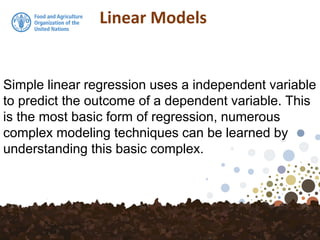
![Linear Models
head(predict(model1))
1 2 3 4 5 6
5.034235 4.757678 3.022235 2.532228 2.502530 3.484401
head(DSM_table$Value)
[1] 11.878804 3.490205 2.317673 1.936148 1.339719 2.285384
head(residuals(model1))
1 2 3 4 5 6
6.8445691 -1.2674728 -0.7045624 -0.5960802 -1.1628119 -1.1990168
head(model2$residuals)
1 2 3 4 5 6
7.3395541 -1.1690560 -0.5363049 -1.2854938 -1.9692882 -1.5173124
> head(model2$fitted.values)
1 2 3 4 5 6
4.539250 4.659261 2.853978 3.221641 3.309007 3.802697](https://image.slidesharecdn.com/d4-2-esp-linear-models-171020070141/85/12-Linear-models-21-320.jpg)
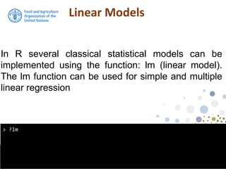
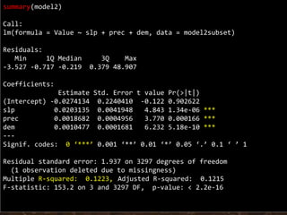
![Multiple regression in R
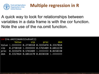
model2subset <-DSM_table2[, c("Value", "slp", "prec", "dem")]
summary(model2subset)
Value slp prec dem
Min. : 0.000 Min. : 0.000 Min. : 424.5 Min. : 45.0
1st Qu.: 1.005 1st Qu.: 0.000 1st Qu.: 532.3 1st Qu.: 404.2
Median : 1.493 Median : 3.000 Median : 564.3 Median : 592.0
Mean : 1.912 Mean : 7.414 Mean : 597.5 Mean : 642.3
3rd Qu.: 2.244 3rd Qu.:11.000 3rd Qu.: 641.8 3rd Qu.: 768.0
Max. :50.332 Max. :56.000 Max. :1180.3 Max. :2375.0
NA's :1
We will regress SOC on Precipitation,
Slope and Elevation. First lets subset these
data out, then get their summary statistics](https://image.slidesharecdn.com/d4-2-esp-linear-models-171020070141/85/12-Linear-models-23-320.jpg)
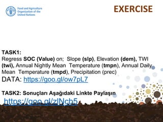
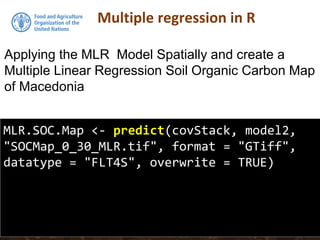

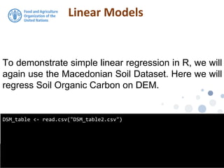
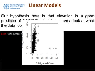
The document discusses the application of linear and multiple regression models in R, particularly using a Macedonian soil dataset to predict soil organic carbon based on elevation, slope, and precipitation. It explains the implementation details of linear models using the 'lm' function, showcasing how to evaluate model fit through summary statistics and residual analysis. The document further includes an exercise for applying these methods to create a spatial soil organic carbon map for Macedonia.
![Reduction of multiple subsystem [compatibility mode]](https://cdn.slidesharecdn.com/ss_thumbnails/reductionofmultiplesubsystemcompatibilitymode-110418075355-phpapp01-thumbnail.jpg?width=640&height=640&fit=bounds)


![Introduction to R for Data Science :: Session 6 [Linear Regression in R]](https://cdn.slidesharecdn.com/ss_thumbnails/intrordatasciencesession6eng-160606173046-thumbnail.jpg?width=640&height=640&fit=bounds)


