Download as PDF, PPTX


![rcdk
• Idioma<c
R
interface
to
the
CDK
library
– I/O
support
for
chemical
file
formats
– Manipula<on
of
atoms,
bonds,
molecules
– Generate
molecular
descriptors,
fingerprints
library(rcdk)
mol <- parse.smiles(‘CCCC’)[[1]]
mols <- load.molecules(‘http://www.rguha.net/mipe100.smi’)](https://image.slidesharecdn.com/bdcon-140913140845-phpapp02/85/Robots-Small-Molecules-R-17-320.jpg)
![rcdk
• rcdk
works
with
references
to
Java
objects
– Can’t
save
them
in
a
workspace
(trivially)
> mol
[1] "Java-Object{AtomContainer(2040919865, #A:4, Atom(2131361171, S:C, H:3,
AtomType(2131361171, FC:0, Isotope(2131361171, Element(2131361171, S:C, AN:6)))),
Atom(1759969037, S:C, H:2, AtomType(1759969037, FC:0, Isotope(1759969037,
Element(1759969037, S:C, AN:6)))), Atom(359851081, S:C, H:2, AtomType(359851081, FC:0,
Isotope(359851081, Element(359851081, S:C, AN:6)))), Atom(703168415, S:C, H:3,
AtomType(703168415, FC:0, Isotope(703168415, Element(703168415, S:C, AN:6)))), #B:3,
Bond(549041464, #O:SINGLE, #S:NONE, #A:2, Atom(2131361171, S:C, H:3,
AtomType(2131361171, FC:0, Isotope(2131361171, Element(2131361171, S:C, AN:6)))),
Atom(1759969037, S:C, H:2, AtomType(1759969037, FC:0, Isotope(1759969037,
Element(1759969037, S:C, AN:6)))), ElectronContainer(549041464EC:2)), Bond(2654289,
#O:SINGLE, #S:NONE, #A:2, Atom(1759969037, S:C, H:2, AtomType(1759969037, FC:0,
Isotope(1759969037, Element(1759969037, S:C, AN:6)))), Atom(359851081, S:C, H:2,
AtomType(359851081, FC:0, Isotope(359851081, Element(359851081, S:C, AN:6)))),
ElectronContainer(2654289EC:2)), Bond(1660962283, #O:SINGLE, #S:NONE, #A:2,
Atom(359851081, S:C, H:2, AtomType(359851081, FC:0, Isotope(359851081,
Element(359851081, S:C, AN:6)))), Atom(703168415, S:C, H:3, AtomType(703168415, FC:0,
Isotope(703168415, Element(703168415, S:C, AN:6)))), ElectronContainer(1660962283EC:
2)))}"
>](https://image.slidesharecdn.com/bdcon-140913140845-phpapp02/85/Robots-Small-Molecules-R-18-320.jpg)


![Calcula<ng
Fingerprints
• Methods
to
compute
similari<es,
generate
summaries
&
manipulate
fingerprints
> fps[[1]]
Fingerprint object
name =
length = 1024
folded = FALSE
source = CDK
bits on = 15 18 45 73 77 78 79 85 87 96 107 109 129 139 149 159
162 166 172 179 194 209 214 223 225 227 239 254 266 272 301 312 327
335 350 354 359 392 393 395 397 415 435 455 486 491 492 499 534 535
541 543 544 545 546 559 575 600 605 618 621 622 626 635 638 644 645
647 690 723 728 742 743 753 754 800 819 831 832 889 893 913 922 930
936 954 985 988 1005 1008 1016
>](https://image.slidesharecdn.com/bdcon-140913140845-phpapp02/85/Robots-Small-Molecules-R-21-320.jpg)


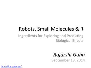
![• Comparison
• Simply
e.g.:
Compare
~
800
solubles
with
>
30k
insolubles
1.0
Use
Case
-‐
Bit
Spectrum
of
two
datasets
is
now
O(n)
take
the
difference
of
the
two
bit
spectra
Frequency
0.5
Normalized 0.0
-0.5
Δ -1.0
Bit Position 0 50 100 150
## make two subsets and generate bit spectra
sol.idx <- which(sol$label == 'high')
insol.idx <- which(sol$label != 'high')
sol.bs <- bit.spectrum(fps[sol.idx])
insol.bs <- bit.spectrum(fps[insol.idx])
## display a difference plot
bsdiff <- sol.bs - insol.bs
d <- data.frame(x=1:length(sol.bs), y=bsdiff)
ggplot(d, aes(x=x,y=y))+geom_line()+
xlab('Bit Position')+
ylab('Normalized Frequency')+
ylim(c(-1,1))](https://image.slidesharecdn.com/bdcon-140913140845-phpapp02/85/Robots-Small-Molecules-R-25-320.jpg)


This document discusses high-throughput screening (HTS) workflows for identifying biologically active small molecules. It describes how robots are used to rapidly screen large libraries of compounds in assays and generate large datasets. Statistical and machine learning methods in R can then be used to build predictive models from these datasets to identify promising leads and guide the screening of additional compounds. Caveats regarding the applicability of models to new chemical spaces are also discussed.