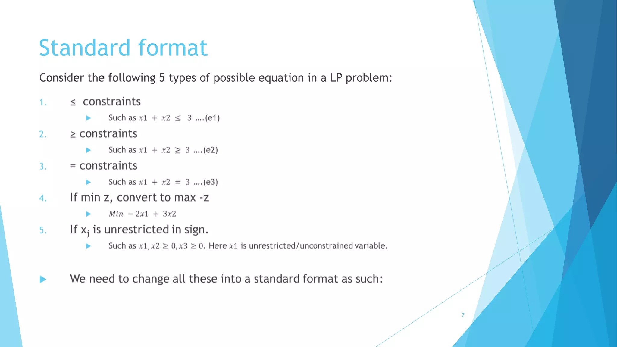
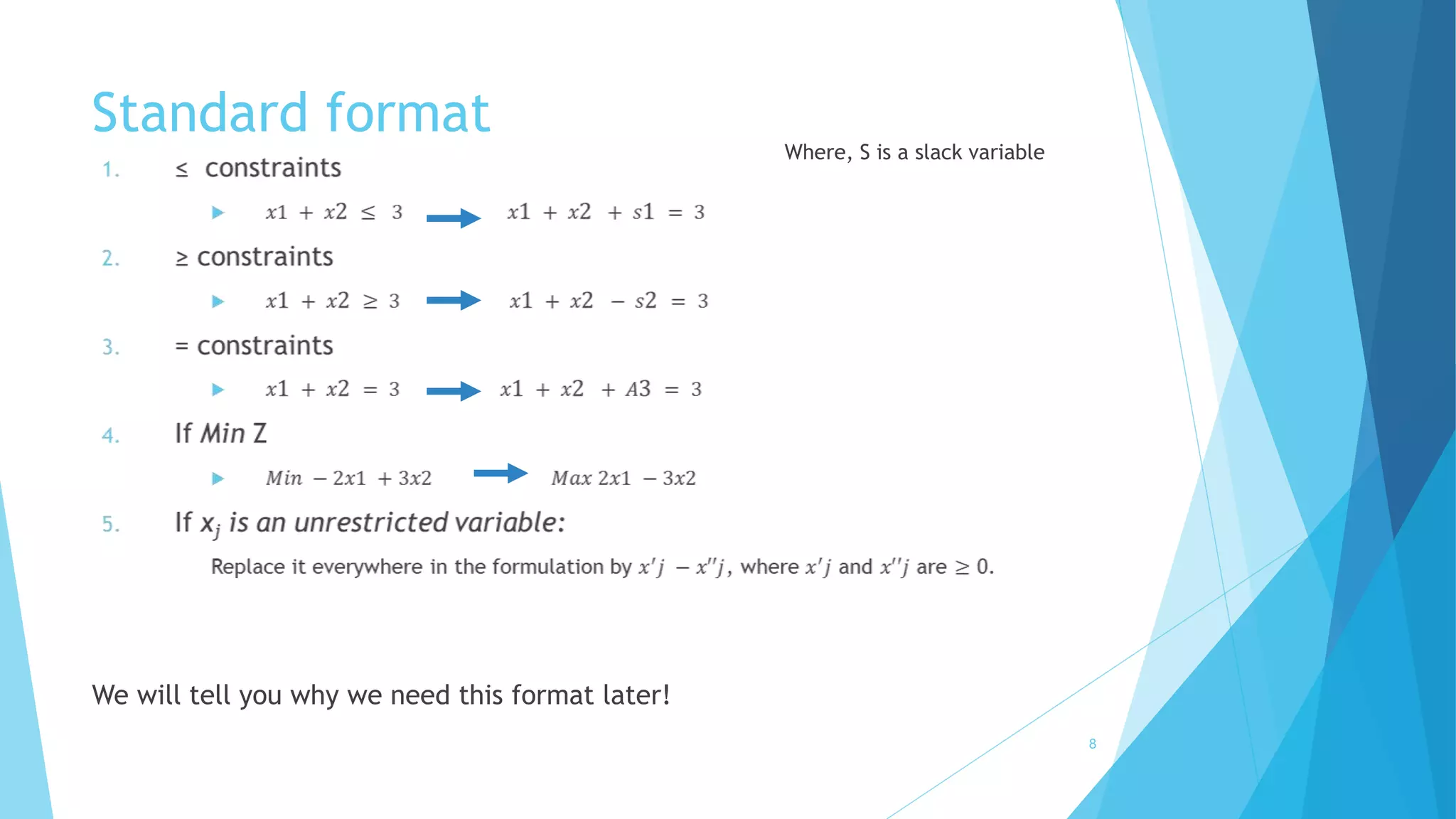
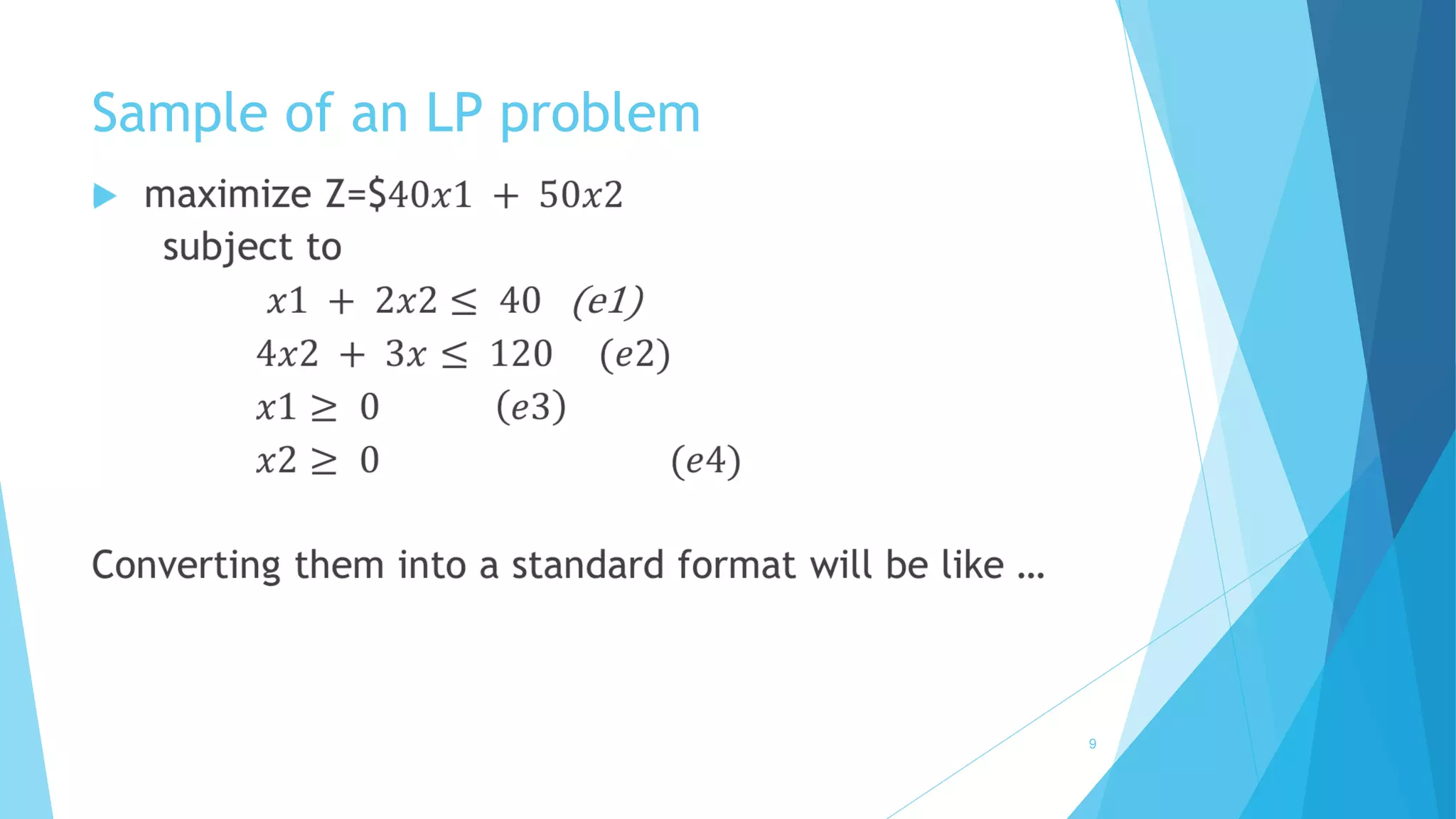
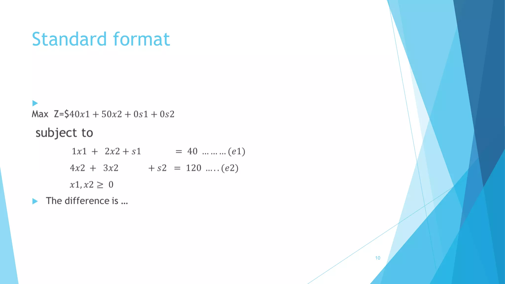
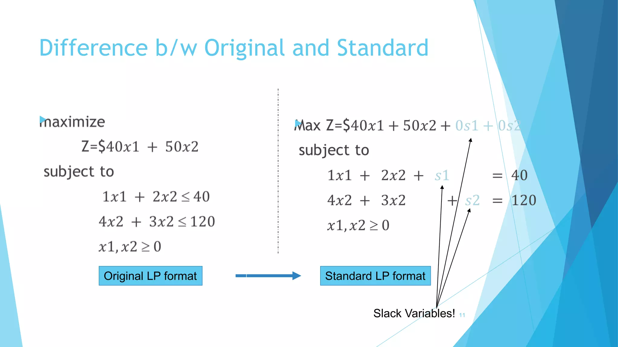
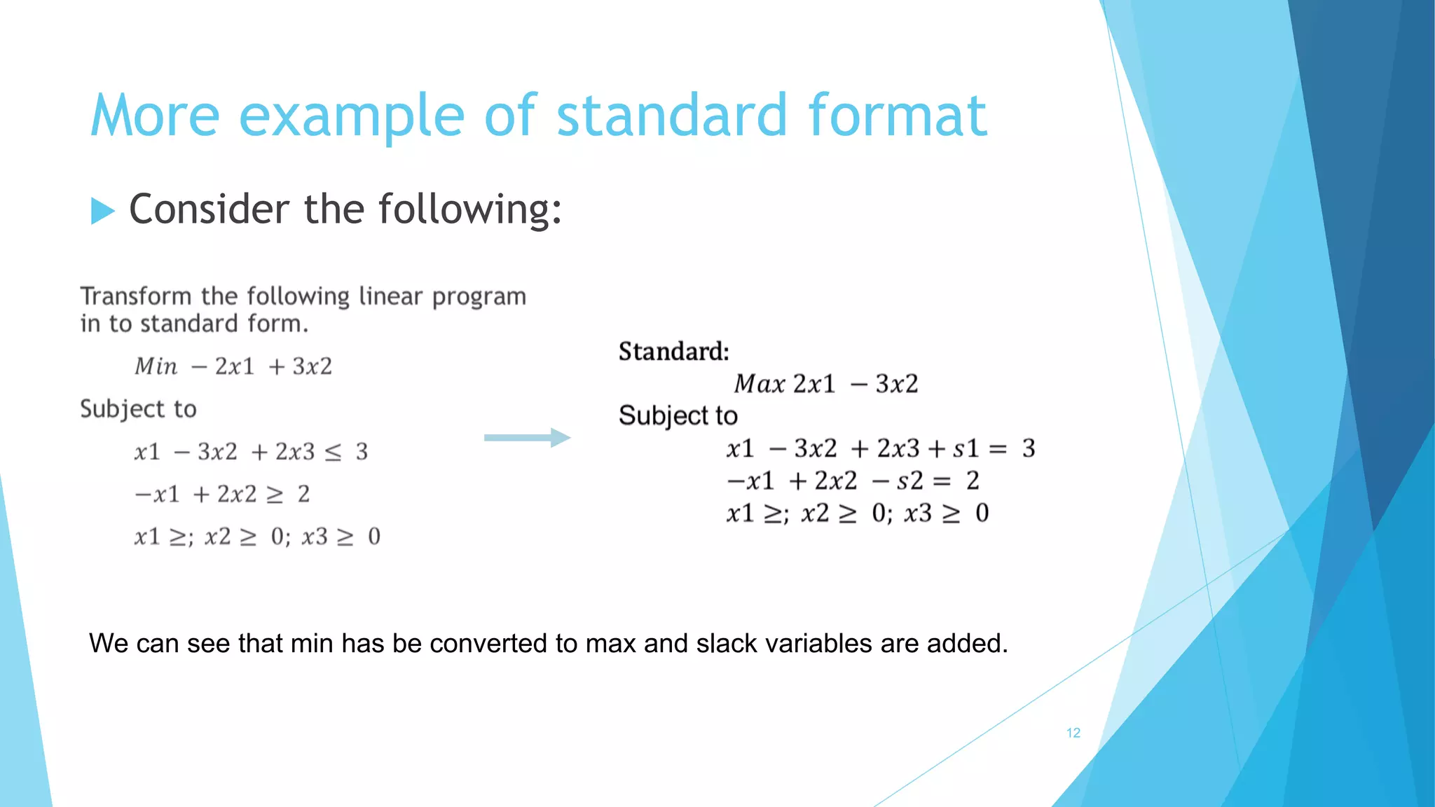
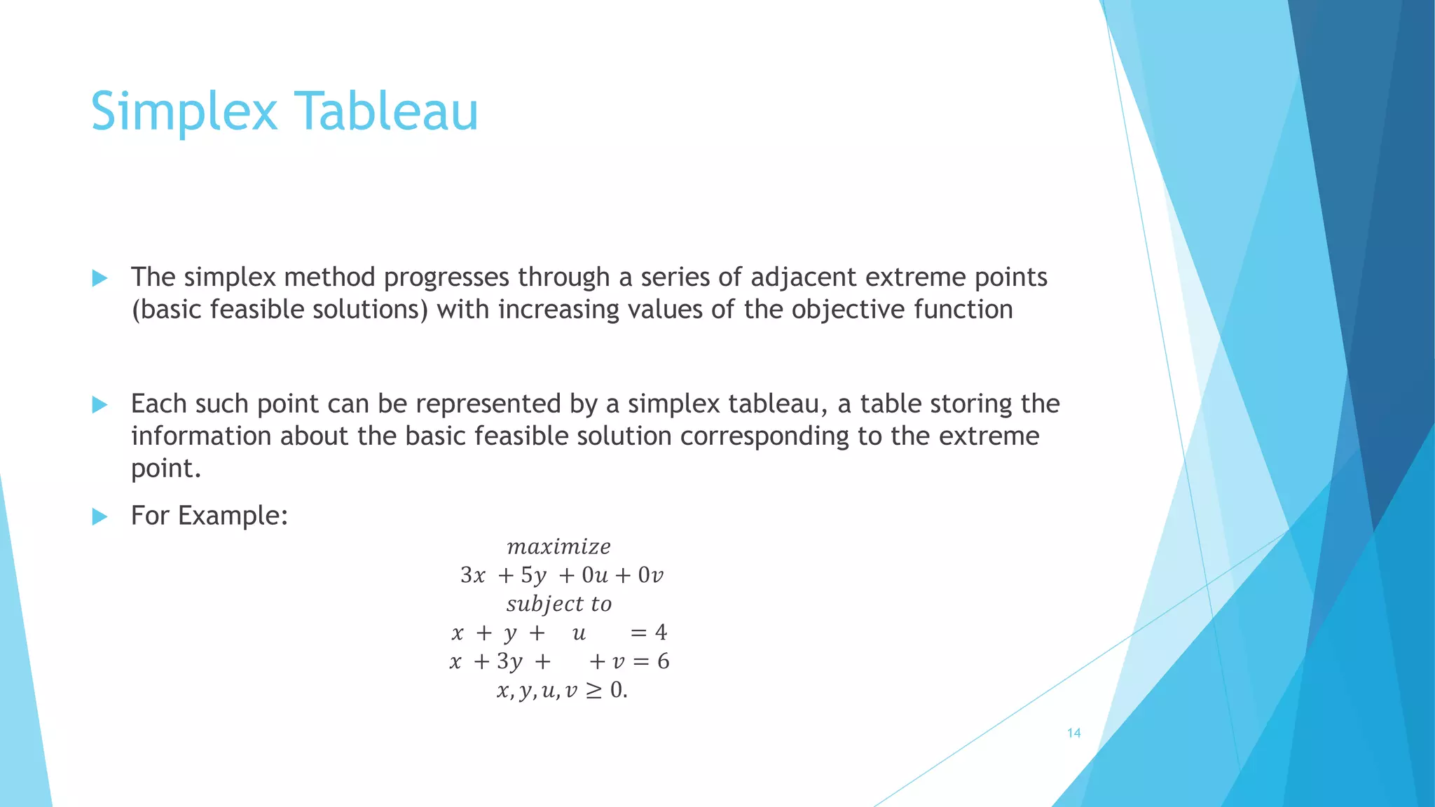
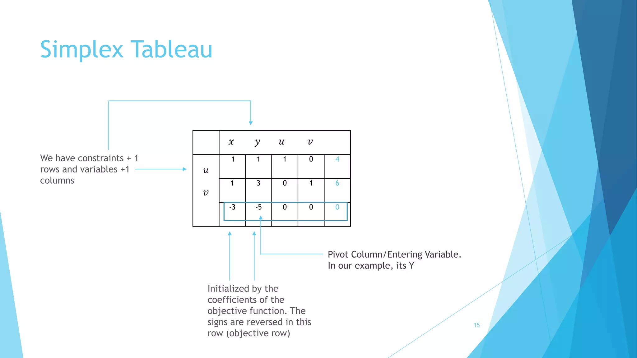
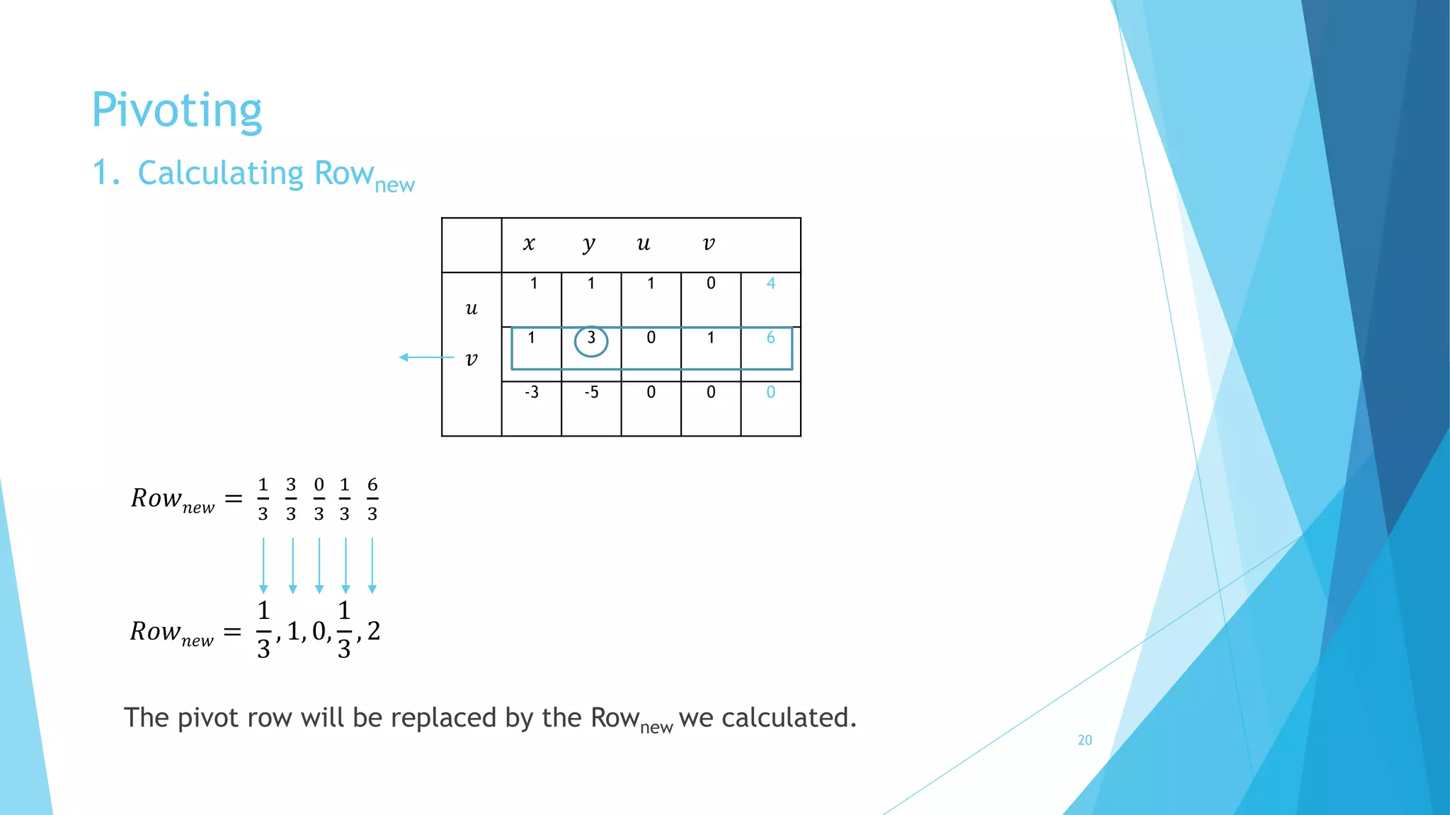
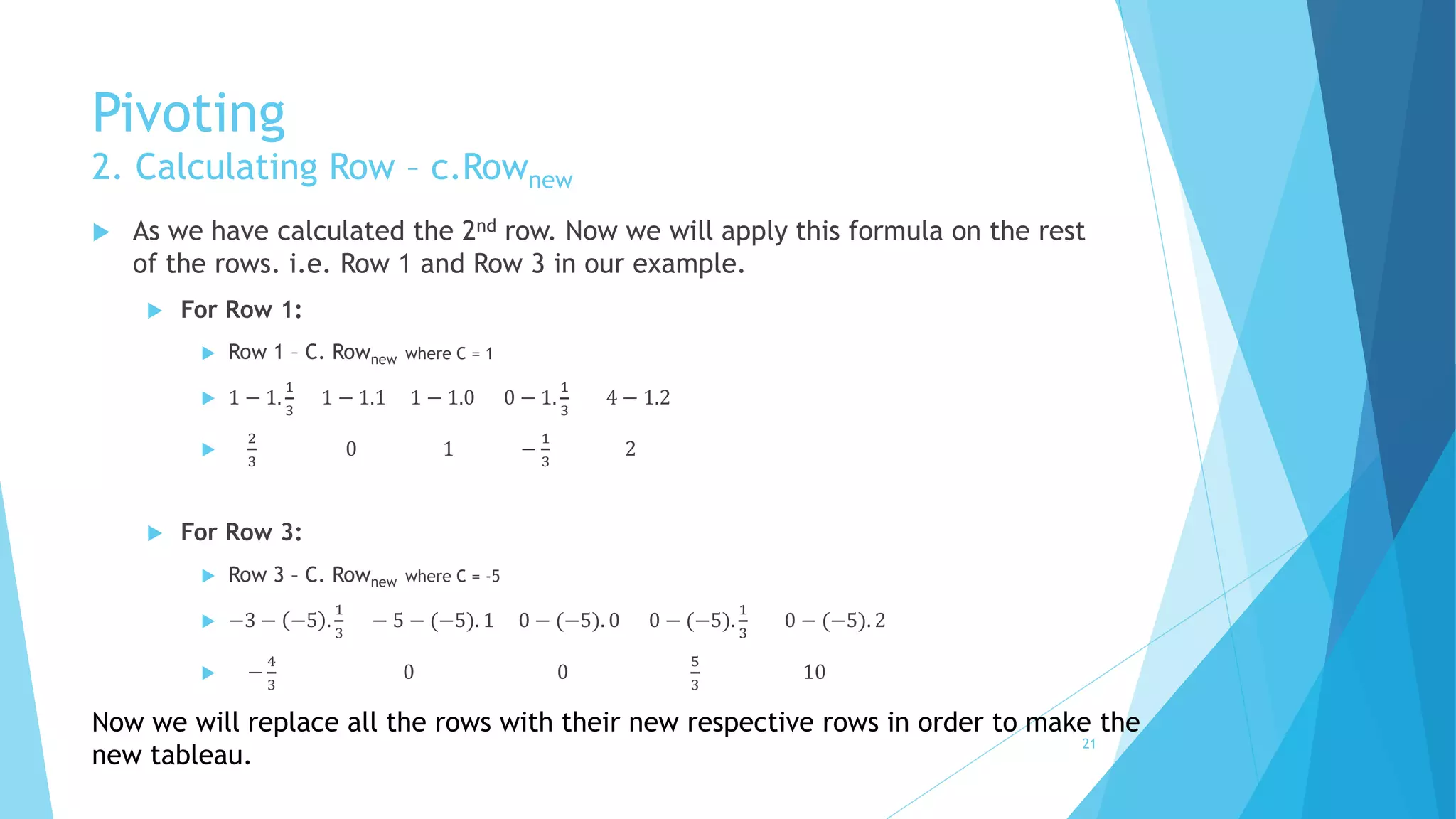
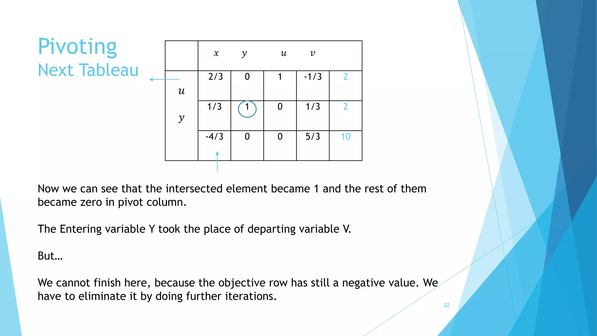
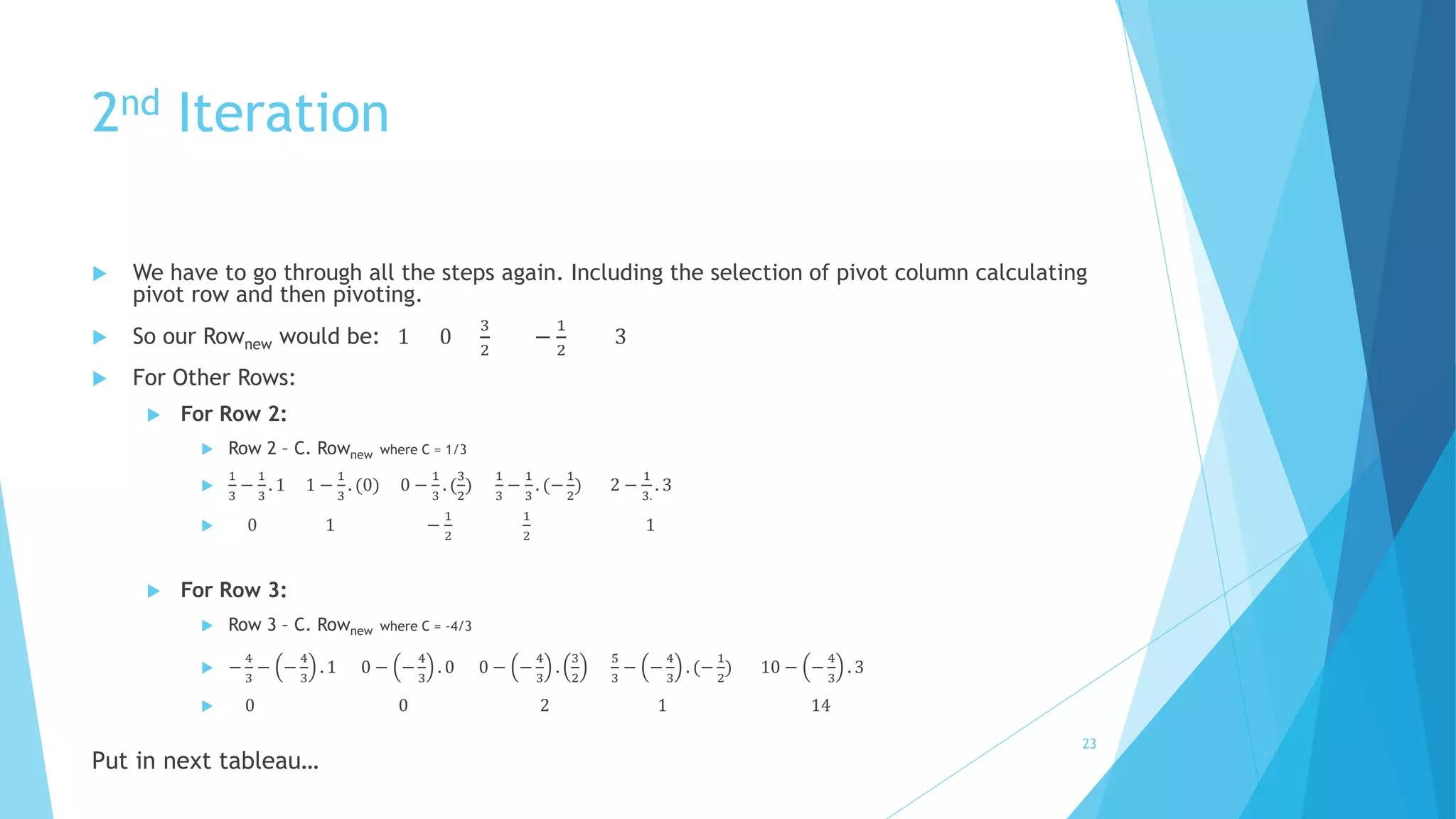
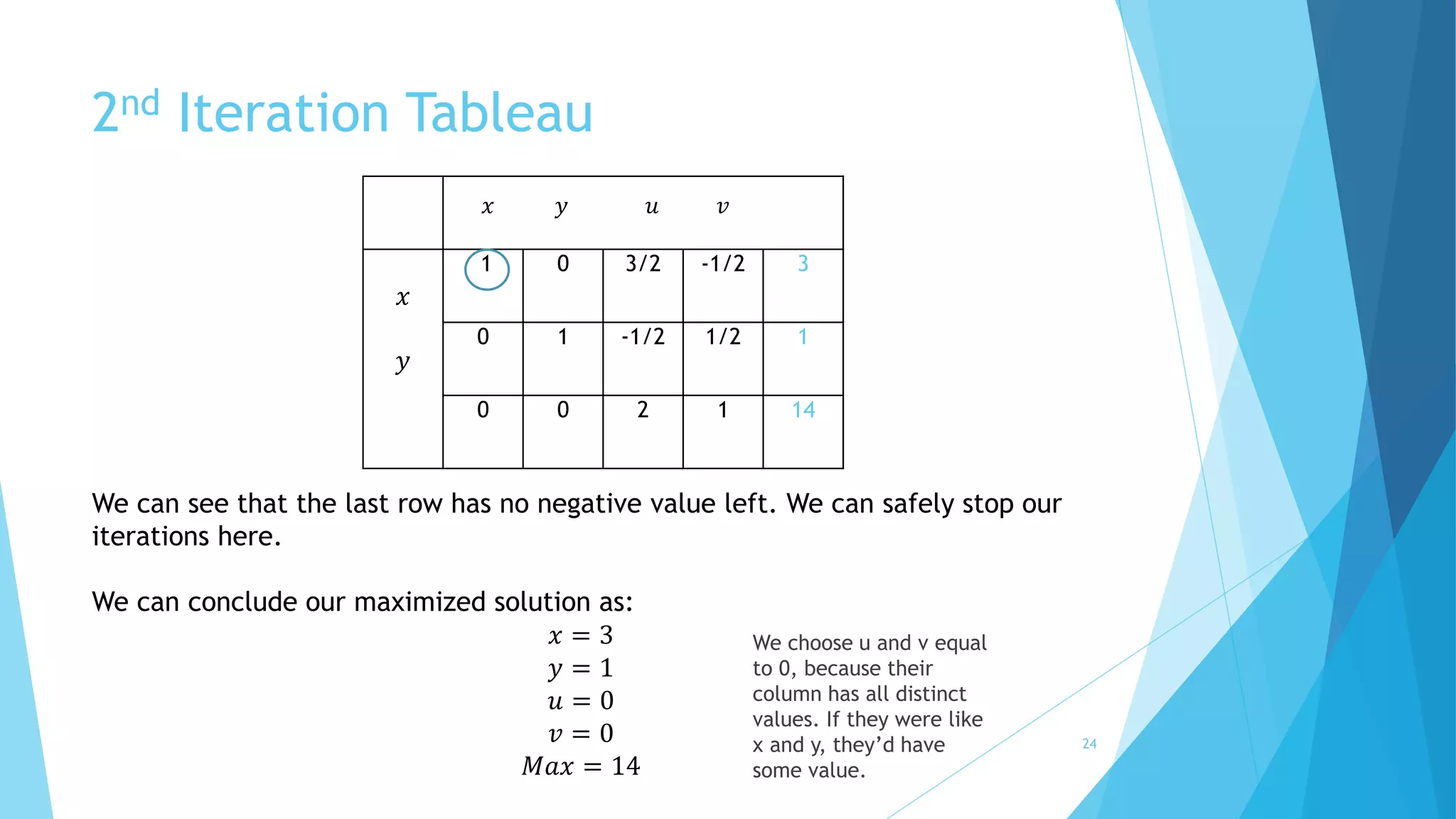
Simplex Algorithm 
Linear Programming 
Khwaja - Sarwan - Aizaz - Ghaffar 
1
Overview 
 Introduction 
 Simplex Algorithm/Method 
 Steps For Simplex Algorithm 
1. Standardization 
2. Simplex Tableau 
3. Pivot Column 
4. Theta Ratio and Pivot Row 
5. Pivoting 
1. Calculate Rownew 
2. Calculate Row – C.Rownew 
 Cycling – Bland’s Rule 
 Software Simulation 
 Efficiency 
 Other Variants of the Algorithm 
 Summary of Algorithm 
 Acknowledgement 2
Simplex Method 
 Last week, we covered on using the graphical approach in deriving solutions 
for LP problem 
 Question: 
 Can we solve all LP problems using graphical approach ? 
3
Answer is “NO” 
 Why? 
 Consider the following scenario: 
15퐶 = 3003) of basic 
For 10 equations with 15 variables there exists a huge number ( 10 
feasible solutions. In such a case, inspection of all the solutions one-by-one is not 
practically feasible. 
 It is extremely difficult to use a graphical approach to find its 
maximized/minimized solution. 
 Thus, we need another systematic approach to solve an LP problem - 
known as Simplex Method/Algorithm. 
4
Simplex Method 
 The most popular method used for the solution of Linear Programming Problems 
(LPP) is the simplex method. 
 The journal Computing in Science and Engineering listed it as one of the top 10 
algorithms of the twentieth century. 
 An American Mathematical Scientist, George Bernard Dantzig is known for his 
development of the simplex algorithm. That’s why we also name it Dantzig’s 
Algorithm. 
 The algorithm is derived from the geometrical concept of Simplex 
(plural simplexes or simplices). 
 Simplex Algorithm can solve an equation for many variables (dimensions). 
5
Steps for Simplex Algorithm 
1. Standardization 
We need to convert our equation into a standard format first. 
We refer standard format here as. 
 It must be a maximization problem. 
 All constraints are in a form of “equation” 
 i.e. not equation of ≥ or ≤ 
 All variables must be required to be nonnegative 
6
Standard format 
7 
Consider the following 5 types of possible equation in a LP problem:
Standard format 
8 
We will tell you why we need this format later! 
Where, S is a slack variable
Sample of an LP problem 
 
9
Standard format 
 
10
Difference b/w Original and Standard 
 
11 
Original LP format Standard LP format 
Slack Variables! 

More example of standard format 
12 
 Consider the following: 
We can see that min has be converted to max and slack variables are added.
2. Simplex Tableau 
13
Simplex Tableau 
 The simplex method progresses through a series of adjacent extreme points 
(basic feasible solutions) with increasing values of the objective function 
 Each such point can be represented by a simplex tableau, a table storing the 
information about the basic feasible solution corresponding to the extreme 
point. 
 For Example: 
푚푎푥푖푚푖푧푒 
3푥 + 5푦 + 0푢 + 0푣 
푠푢푏푗푒푐푡 푡표 
푥 + 푦 + 푢 = 4 
푥 + 3푦 + + 푣 = 6 
푥, 푦, 푢, 푣 ≥ 0. 
14
Simplex Tableau 
푢 
푣 
푥 푦 푢 푣 
1 1 1 0 4 
1 3 0 1 6 
-3 -5 0 0 0 
Initialized by the 
coefficients of the 
objective function. The 
signs are reversed in this 
row (objective row) 
We have constraints + 1 
rows and variables +1 
columns 
Pivot Column/Entering Variable. 
In our example, its Y 
15
Simplex Tableau 
3.Pivot Column 
 Objective Row: 
 The objective row is used by the simplex method to check whether the current 
tableau represents an optimal solution. 
 It does have the optimum solution if all the entries in the objective row—except, possibly, 
the one in the last column—are nonnegative. 
 Pivot Column/Entering Variable: 
 Select the minimum number in the objective row, such a choice yields the largest 
increase in the objective function’s value per unit of change in a variable’s value. 
The most negative one selected will be the pivot column with an entering variable. 
It is indicated by the up arrow. 
16
Simplex Tableau 
4. Calculating the Theta Ratio and Departing Variable 
 Departing Variable: 
 Also called leaving variable or pivot row i.e., a basic variable to become non basic 
in the next tableau. Indicated by 
 How to calculate: 
 For each positive entry in the pivot column, compute the θ-ratio by dividing the 
row’s last entry by the entry in the pivot column. 
 The row with the smallest θ-ratio determines the departing variable, i.e., the 
variable to become non basic. 
 If there are no positive entries in the pivot column, no θ-ratio can be computed, 
which indicates that the problem is unbounded and the algorithm stops. 
17
Simplex Tableau 
Calculating the Theta Ratio and Departing Variable 
푢 
푣 
푥 푦 푢 푣 
1 1 1 0 4 
1 3 0 1 6 
-3 -5 0 0 0 
Pivot Column/Entering Variable 
휃 − 푟푎푡푖표 = 
4 
1 
= 4 
휃 − 푟푎푡푖표 = 
6 
3 
= 2 
The row with the smallest θ-ratio determines the 
departing variable. For our example, it is variable v. 
The intersecting element of Pivot Column and Pivot 
Row is the pivot. 
In the next tableau the intersected element will 
become 1 and the rest of elements will become 0 in 
the pivot column. 
Departing Variable / Leaving Variable/ Pivot Row 
18
5. Pivoting 
 To transform the current tableau into the next one and increase the value of 
the objective function to the next feasible solution. We have to take some 
steps. Called Pivoting 
 Pivoting, is similar to the principal step of the Gauss-Jordan elimination 
algorithm for solving systems of linear equations. 
 Steps: 
1. First, divide all the entries of the pivot row by the pivot, its entry in the pivot 
column, to obtain Rownew 
2. Then, replace each of the other rows, including the objective row, by the 
difference 
 푅표푤 − 푐. 푅표푤푛푒푤 
 Where c is the row’s entry in the pivot column. 
19
Pivoting 
1. Calculating Rownew 
푢 
푣 
푥 푦 푢 푣 
1 1 1 0 4 
1 3 0 1 6 
-3 -5 0 0 0 
푅표푤푛푒푤 = 
1 
3 
3 
3 
0 
3 
1 
3 
6 
3 
푅표푤푛푒푤 = 
1 
3 
, 1, 0, 
1 
3 
, 2 
The pivot row will be replaced by the Rownew we calculated. 
20
Pivoting 
2. Calculating Row – c.Rownew 
 As we have calculated the 2nd row. Now we will apply this formula on the rest 
of the rows. i.e. Row 1 and Row 3 in our example. 
 For Row 1: 
 Row 1 – C. Rownew where C = 1 
 1 − 1. 
1 
3 
1 − 1.1 1 − 1.0 0 − 1. 
1 
3 
4 − 1.2 
 
2 
3 
0 1 − 
1 
3 
2 
 For Row 3: 
 Row 3 – C. Rownew where C = -5 
 −3 − −5 . 
1 
3 
− 5 − (−5). 1 0 − (−5). 0 0 − (−5). 
1 
3 
0 − (−5). 2 
 − 
4 
3 
0 0 
5 
3 
10 
Now we will replace all the rows with their new respective rows in order to make the 
new tableau. 21
Pivoting 
Next Tableau 
푢 
푦 
푥 푦 푢 푣 
2/3 0 1 -1/3 2 
1/3 1 0 1/3 2 
-4/3 0 0 5/3 10 
Now we can see that the intersected element became 1 and the rest of them 
became zero in pivot column. 
The Entering variable Y took the place of departing variable V. 
But… 
We cannot finish here, because the objective row has still a negative value. We 
have to eliminate it by doing further iterations. 
22
2nd Iteration 
 We have to go through all the steps again. Including the selection of pivot column calculating 
pivot row and then pivoting. 
 So our Rownew would be: 1 0 
3 
2 
− 
1 
2 
3 
 For Other Rows: 
 For Row 2: 
 Row 2 – C. Rownew where C = 1/3 
 
1 
3 
− 
1 
3 
. 1 1 − 
1 
3 
. (0) 0 − 
1 
3 
. ( 
3 
2 
) 
1 
3 
− 
1 
3 
. (− 
1 
2 
) 2 − 
1 
3. 
. 3 
 0 1 − 
1 
2 
1 
2 
1 
 For Row 3: 
 Row 3 – C. Rownew where C = -4/3 
 − 
4 
3 
− − 
4 
3 
. 1 0 − − 
4 
3 
. 0 0 − − 
4 
3 
. 
3 
2 
5 
3 
− − 
4 
3 
. (− 
1 
2 
) 10 − − 
4 
3 
. 3 
 0 0 2 1 14 
Put in next tableau… 
23
2nd Iteration Tableau 
푥 
푦 
푥 푦 푢 푣 
1 0 3/2 -1/2 3 
0 1 -1/2 1/2 1 
0 0 2 1 14 
We can see that the last row has no negative value left. We can safely stop our 
iterations here. 
We can conclude our maximized solution as: 
푥 = 3 
푦 = 1 
푢 = 0 
푣 = 0 
푀푎푥 = 14 
We choose u and v equal 
to 0, because their 
column has all distinct 
values. If they were like 
x and y, they’d have 
some value. 
24
Cycling – Bland’s Rule 
 When an objective function’s values “stall” for several iterations in a row and 
that the algorithm cycles back to a previously considered point and hence 
never terminate. This phenomenon is called cycling. 
 Although, it rarely happens, but when it does - A simple modification of the 
simplex method, called Bland’s rule, eliminates even the theoretical 
possibility of cycling. 
25
Cycling – Bland’s Rule 
 Assuming that the variables are denoted by a subscripted letter (e.g., x1, 
x2,..., xn), this rule can be stated as follows: 
1. Among the columns with a negative entry in the objective row, select the 
column with the smallest subscript. 
2. Resolve a tie among the smallest θ-ratios by selecting the row labeled by the 
basic variable with the smallest subscript. 
26
Software Simulation 
 Simplex Method has became so efficient that its calculation packages are 
even available online. One of them is as follows: 
 For ease, we will copy the same problem to the online tool and check 
whether it gives us the same result: 
maximize p = 3x +5y 
subject to x + y = 4, x+3y = 6 
 Simplex Method Online Tool 
27
Efficiency 
How efficient is the simplex method? 
28
Efficiency of Simplex Algorithm 
 Since we know that the algorithm progresses through a sequence of adjacent 
points of a feasible region. Right? 
 So, one should probably expect bad news because the number of extreme 
points is known to grow exponentially with the problem size. 
 The worst-case efficiency of the simplex method has been shown to be 
exponential. 
 But Fortunately! 
 More than half a century of practical experience with the algorithm has 
shown that the number of iterations in a typical application ranges between 
m and 3m, with the number of operations per iteration proportional to mn, 
where m and n are the numbers of equality constraints and variables, 
respectively. 
29
Other Variants of the Algorithm 
 Ellipsoid Method: 
 An important mile- stone in the history of such algorithms was the proof by L. G. 
Khachian showing that the ellipsoid method can solve any linear programming 
problem in polynomial time. 
 However, ellipsoid method was much slower than the simplex method in practice 
 Karmarker’s Method 
 Narendra Karmarkar published an algorithm that not only had a polynomial worst-case 
efficiency but also was competitive with the simplex method. This method 
generates a sequence of feasible solutions that lie within the feasible region 
rather than going through a sequence of adjacent extreme points as the simplex 
method does. (Interior Point Methods). 
30
Summary of Simplex Algorithm 
 Step 0 
 Initialization. Present a given linear programming problem in standard form and set up an initial 
tableau with non negative entries in the rightmost column. 
 Step 1 
 Optimality test. If all the entries in the objective row are nonnegative—stop: the tableau 
represents an optimal solution whose basic variables’ values are in the rightmost column and 
the remaining, non basic variables’ values are zeros. 
 Step 3 
 Finding the entering variable. Select the most negative entry from among the first n elements 
of the objective row. 
 Step 4 
 Finding the departing variable. For each positive entry in the pivot column, calculate the θ- 
ratio. Find the row with the smallest θ-ratio. 
 Step 5 
 Forming the next tableau. Divide all the entries in the pivot row by its entry in the pivot 
column. Subtract from each of the other rows, including the objective row, the new pivot row 
multiplied by the entry in the pivot column of the row in question. (This will make all the 
entries in the pivot column 0’s except for 1in the pivot row.) Replace the label of the pivot row 
by the variable’s name of the pivot column and go back to Step 1. 31
Acknowledgment 
The material presented in this lecture is adopted from; Anany Levitin. 
Introduction to Design and Analysis of Algorithms, 3rd Edition 
32
Thank You! 
33

Simplex algorithm

  • 1.
    Simplex Algorithm LinearProgramming Khwaja - Sarwan - Aizaz - Ghaffar 1
  • 2.
    Overview  Introduction  Simplex Algorithm/Method  Steps For Simplex Algorithm 1. Standardization 2. Simplex Tableau 3. Pivot Column 4. Theta Ratio and Pivot Row 5. Pivoting 1. Calculate Rownew 2. Calculate Row – C.Rownew  Cycling – Bland’s Rule  Software Simulation  Efficiency  Other Variants of the Algorithm  Summary of Algorithm  Acknowledgement 2
  • 3.
    Simplex Method Last week, we covered on using the graphical approach in deriving solutions for LP problem  Question:  Can we solve all LP problems using graphical approach ? 3
  • 4.
    Answer is “NO”  Why?  Consider the following scenario: 15퐶 = 3003) of basic For 10 equations with 15 variables there exists a huge number ( 10 feasible solutions. In such a case, inspection of all the solutions one-by-one is not practically feasible.  It is extremely difficult to use a graphical approach to find its maximized/minimized solution.  Thus, we need another systematic approach to solve an LP problem - known as Simplex Method/Algorithm. 4
  • 5.
    Simplex Method The most popular method used for the solution of Linear Programming Problems (LPP) is the simplex method.  The journal Computing in Science and Engineering listed it as one of the top 10 algorithms of the twentieth century.  An American Mathematical Scientist, George Bernard Dantzig is known for his development of the simplex algorithm. That’s why we also name it Dantzig’s Algorithm.  The algorithm is derived from the geometrical concept of Simplex (plural simplexes or simplices).  Simplex Algorithm can solve an equation for many variables (dimensions). 5
  • 6.
    Steps for SimplexAlgorithm 1. Standardization We need to convert our equation into a standard format first. We refer standard format here as.  It must be a maximization problem.  All constraints are in a form of “equation”  i.e. not equation of ≥ or ≤  All variables must be required to be nonnegative 6
  • 7.
    Standard format 7 Consider the following 5 types of possible equation in a LP problem:
  • 8.
    Standard format 8 We will tell you why we need this format later! Where, S is a slack variable
  • 9.
    Sample of anLP problem  9
  • 10.
  • 11.
    Difference b/w Originaland Standard  11 Original LP format Standard LP format Slack Variables! 
  • 12.
    More example ofstandard format 12  Consider the following: We can see that min has be converted to max and slack variables are added.
  • 13.
  • 14.
    Simplex Tableau The simplex method progresses through a series of adjacent extreme points (basic feasible solutions) with increasing values of the objective function  Each such point can be represented by a simplex tableau, a table storing the information about the basic feasible solution corresponding to the extreme point.  For Example: 푚푎푥푖푚푖푧푒 3푥 + 5푦 + 0푢 + 0푣 푠푢푏푗푒푐푡 푡표 푥 + 푦 + 푢 = 4 푥 + 3푦 + + 푣 = 6 푥, 푦, 푢, 푣 ≥ 0. 14
  • 15.
    Simplex Tableau 푢 푣 푥 푦 푢 푣 1 1 1 0 4 1 3 0 1 6 -3 -5 0 0 0 Initialized by the coefficients of the objective function. The signs are reversed in this row (objective row) We have constraints + 1 rows and variables +1 columns Pivot Column/Entering Variable. In our example, its Y 15
  • 16.
    Simplex Tableau 3.PivotColumn  Objective Row:  The objective row is used by the simplex method to check whether the current tableau represents an optimal solution.  It does have the optimum solution if all the entries in the objective row—except, possibly, the one in the last column—are nonnegative.  Pivot Column/Entering Variable:  Select the minimum number in the objective row, such a choice yields the largest increase in the objective function’s value per unit of change in a variable’s value. The most negative one selected will be the pivot column with an entering variable. It is indicated by the up arrow. 16
  • 17.
    Simplex Tableau 4.Calculating the Theta Ratio and Departing Variable  Departing Variable:  Also called leaving variable or pivot row i.e., a basic variable to become non basic in the next tableau. Indicated by  How to calculate:  For each positive entry in the pivot column, compute the θ-ratio by dividing the row’s last entry by the entry in the pivot column.  The row with the smallest θ-ratio determines the departing variable, i.e., the variable to become non basic.  If there are no positive entries in the pivot column, no θ-ratio can be computed, which indicates that the problem is unbounded and the algorithm stops. 17
  • 18.
    Simplex Tableau Calculatingthe Theta Ratio and Departing Variable 푢 푣 푥 푦 푢 푣 1 1 1 0 4 1 3 0 1 6 -3 -5 0 0 0 Pivot Column/Entering Variable 휃 − 푟푎푡푖표 = 4 1 = 4 휃 − 푟푎푡푖표 = 6 3 = 2 The row with the smallest θ-ratio determines the departing variable. For our example, it is variable v. The intersecting element of Pivot Column and Pivot Row is the pivot. In the next tableau the intersected element will become 1 and the rest of elements will become 0 in the pivot column. Departing Variable / Leaving Variable/ Pivot Row 18
  • 19.
    5. Pivoting To transform the current tableau into the next one and increase the value of the objective function to the next feasible solution. We have to take some steps. Called Pivoting  Pivoting, is similar to the principal step of the Gauss-Jordan elimination algorithm for solving systems of linear equations.  Steps: 1. First, divide all the entries of the pivot row by the pivot, its entry in the pivot column, to obtain Rownew 2. Then, replace each of the other rows, including the objective row, by the difference  푅표푤 − 푐. 푅표푤푛푒푤  Where c is the row’s entry in the pivot column. 19
  • 20.
    Pivoting 1. CalculatingRownew 푢 푣 푥 푦 푢 푣 1 1 1 0 4 1 3 0 1 6 -3 -5 0 0 0 푅표푤푛푒푤 = 1 3 3 3 0 3 1 3 6 3 푅표푤푛푒푤 = 1 3 , 1, 0, 1 3 , 2 The pivot row will be replaced by the Rownew we calculated. 20
  • 21.
    Pivoting 2. CalculatingRow – c.Rownew  As we have calculated the 2nd row. Now we will apply this formula on the rest of the rows. i.e. Row 1 and Row 3 in our example.  For Row 1:  Row 1 – C. Rownew where C = 1  1 − 1. 1 3 1 − 1.1 1 − 1.0 0 − 1. 1 3 4 − 1.2  2 3 0 1 − 1 3 2  For Row 3:  Row 3 – C. Rownew where C = -5  −3 − −5 . 1 3 − 5 − (−5). 1 0 − (−5). 0 0 − (−5). 1 3 0 − (−5). 2  − 4 3 0 0 5 3 10 Now we will replace all the rows with their new respective rows in order to make the new tableau. 21
  • 22.
    Pivoting Next Tableau 푢 푦 푥 푦 푢 푣 2/3 0 1 -1/3 2 1/3 1 0 1/3 2 -4/3 0 0 5/3 10 Now we can see that the intersected element became 1 and the rest of them became zero in pivot column. The Entering variable Y took the place of departing variable V. But… We cannot finish here, because the objective row has still a negative value. We have to eliminate it by doing further iterations. 22
  • 23.
    2nd Iteration We have to go through all the steps again. Including the selection of pivot column calculating pivot row and then pivoting.  So our Rownew would be: 1 0 3 2 − 1 2 3  For Other Rows:  For Row 2:  Row 2 – C. Rownew where C = 1/3  1 3 − 1 3 . 1 1 − 1 3 . (0) 0 − 1 3 . ( 3 2 ) 1 3 − 1 3 . (− 1 2 ) 2 − 1 3. . 3  0 1 − 1 2 1 2 1  For Row 3:  Row 3 – C. Rownew where C = -4/3  − 4 3 − − 4 3 . 1 0 − − 4 3 . 0 0 − − 4 3 . 3 2 5 3 − − 4 3 . (− 1 2 ) 10 − − 4 3 . 3  0 0 2 1 14 Put in next tableau… 23
  • 24.
    2nd Iteration Tableau 푥 푦 푥 푦 푢 푣 1 0 3/2 -1/2 3 0 1 -1/2 1/2 1 0 0 2 1 14 We can see that the last row has no negative value left. We can safely stop our iterations here. We can conclude our maximized solution as: 푥 = 3 푦 = 1 푢 = 0 푣 = 0 푀푎푥 = 14 We choose u and v equal to 0, because their column has all distinct values. If they were like x and y, they’d have some value. 24
  • 25.
    Cycling – Bland’sRule  When an objective function’s values “stall” for several iterations in a row and that the algorithm cycles back to a previously considered point and hence never terminate. This phenomenon is called cycling.  Although, it rarely happens, but when it does - A simple modification of the simplex method, called Bland’s rule, eliminates even the theoretical possibility of cycling. 25
  • 26.
    Cycling – Bland’sRule  Assuming that the variables are denoted by a subscripted letter (e.g., x1, x2,..., xn), this rule can be stated as follows: 1. Among the columns with a negative entry in the objective row, select the column with the smallest subscript. 2. Resolve a tie among the smallest θ-ratios by selecting the row labeled by the basic variable with the smallest subscript. 26
  • 27.
    Software Simulation Simplex Method has became so efficient that its calculation packages are even available online. One of them is as follows:  For ease, we will copy the same problem to the online tool and check whether it gives us the same result: maximize p = 3x +5y subject to x + y = 4, x+3y = 6  Simplex Method Online Tool 27
  • 28.
    Efficiency How efficientis the simplex method? 28
  • 29.
    Efficiency of SimplexAlgorithm  Since we know that the algorithm progresses through a sequence of adjacent points of a feasible region. Right?  So, one should probably expect bad news because the number of extreme points is known to grow exponentially with the problem size.  The worst-case efficiency of the simplex method has been shown to be exponential.  But Fortunately!  More than half a century of practical experience with the algorithm has shown that the number of iterations in a typical application ranges between m and 3m, with the number of operations per iteration proportional to mn, where m and n are the numbers of equality constraints and variables, respectively. 29
  • 30.
    Other Variants ofthe Algorithm  Ellipsoid Method:  An important mile- stone in the history of such algorithms was the proof by L. G. Khachian showing that the ellipsoid method can solve any linear programming problem in polynomial time.  However, ellipsoid method was much slower than the simplex method in practice  Karmarker’s Method  Narendra Karmarkar published an algorithm that not only had a polynomial worst-case efficiency but also was competitive with the simplex method. This method generates a sequence of feasible solutions that lie within the feasible region rather than going through a sequence of adjacent extreme points as the simplex method does. (Interior Point Methods). 30
  • 31.
    Summary of SimplexAlgorithm  Step 0  Initialization. Present a given linear programming problem in standard form and set up an initial tableau with non negative entries in the rightmost column.  Step 1  Optimality test. If all the entries in the objective row are nonnegative—stop: the tableau represents an optimal solution whose basic variables’ values are in the rightmost column and the remaining, non basic variables’ values are zeros.  Step 3  Finding the entering variable. Select the most negative entry from among the first n elements of the objective row.  Step 4  Finding the departing variable. For each positive entry in the pivot column, calculate the θ- ratio. Find the row with the smallest θ-ratio.  Step 5  Forming the next tableau. Divide all the entries in the pivot row by its entry in the pivot column. Subtract from each of the other rows, including the objective row, the new pivot row multiplied by the entry in the pivot column of the row in question. (This will make all the entries in the pivot column 0’s except for 1in the pivot row.) Replace the label of the pivot row by the variable’s name of the pivot column and go back to Step 1. 31
  • 32.
    Acknowledgment The materialpresented in this lecture is adopted from; Anany Levitin. Introduction to Design and Analysis of Algorithms, 3rd Edition 32
  • 33.