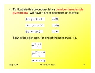
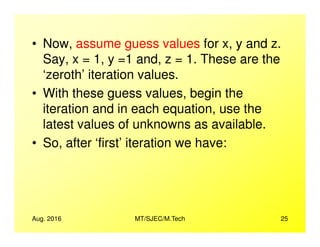
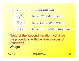
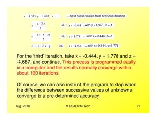
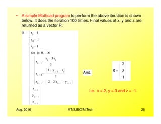
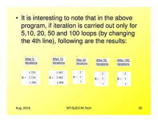
This document discusses numerical methods for solving steady-state 1D and 2D heat conduction problems. It describes the relaxation method, Gaussian elimination method, and Gauss-Siedel iteration method for solving systems of simultaneous algebraic equations arising in heat conduction analyses. The Gaussian elimination and matrix inversion methods use matrix operations to systematically eliminate variables. The Gauss-Siedel iteration method iteratively solves for each variable using the most recently calculated values of other variables until convergence is reached. Examples are provided to illustrate each numerical solution technique.
KIT-601 Lecture Notes-UNIT-3.pdf Mining Data Stream
NUMERICAL METHODS IN STEADY STATE, 1D and 2D HEAT CONDUCTION- Part-II
1. Lectures on Heat Transfer --
NUMERICAL METHODS IN STEADY
STATE 1D and 2D HEAT
CONDUCTION – Part-II
by
Dr. M. ThirumaleshwarDr. M. Thirumaleshwar
formerly:
Professor, Dept. of Mechanical Engineering,
St. Joseph Engg. College, Vamanjoor,
Mangalore,
India
2. Preface
• This file contains slides on NUMERICAL
METHODS IN STEADY STATE 1D and 2D
HEAT CONDUCTION – Part-II.
• The slides were prepared while teaching
Heat Transfer course to the M.Tech.Heat Transfer course to the M.Tech.
students in Mechanical Engineering Dept.
of St. Joseph Engineering College,
Vamanjoor, Mangalore, India, during Sept.
– Dec. 2010.
Aug. 2016 2MT/SJEC/M.Tech
3. • It is hoped that these Slides will be useful
to teachers, students, researchers and
professionals working in this field.
• For students, it should be particularly
useful to study, quickly review the subject,useful to study, quickly review the subject,
and to prepare for the examinations.
•
Aug. 2016 3MT/SJEC/M.Tech
4. References:
• 1. M. Thirumaleshwar: Fundamentals of Heat &
Mass Transfer, Pearson Edu., 2006
• https://books.google.co.in/books?id=b2238B-
AsqcC&printsec=frontcover&source=gbs_atb#v=onepage&q&f=false
• 2. Cengel Y. A. Heat Transfer: A Practical
Approach, 2nd Ed. McGraw Hill Co., 2003
Aug. 2016 MT/SJEC/M.Tech 4
Approach, 2nd Ed. McGraw Hill Co., 2003
• 3. Cengel, Y. A. and Ghajar, A. J., Heat and
Mass Transfer - Fundamentals and Applications,
5th Ed., McGraw-Hill, New York, NY, 2014.
5. References… contd.
• 4. Incropera , Dewitt, Bergman, Lavine:
Fundamentals of Heat and Mass Transfer, 6th
Ed., Wiley Intl.
• 5. M. Thirumaleshwar: Software Solutions to• 5. M. Thirumaleshwar: Software Solutions to
Problems on Heat Transfer – CONDUCTION-
Part-II, Bookboon, 2013
• http://bookboon.com/en/software-solutions-problems-on-heat-
transfer-cii-ebook
Aug. 2016 MT/SJEC/M.Tech 5
6. NUMERICAL METHODS IN STEADY STATE 1D
and 2D HEAT CONDUCTION- Part-II
• Methods of solving a system of
simultaneous, algebraic equations - 1D
steady state conduction in cylindrical and
spherical systems - 2D steady state
Aug. 2016 MT/SJEC/M.Tech 6
spherical systems - 2D steady state
conduction in cartesian coordinates -
Problems
7. Methods of solving a system of
simultaneous, algebraic equations:
• We shall briefly present a few methods:
• Relaxation method
• Direct methods: (a) Gaussian
elimination, and (b) Matrix inversion
Aug. 2016 MT/SJEC/M.Tech 7
elimination, and (b) Matrix inversion
• Iterative methods: e.g. Gauss – Siedel
iteration method
8. • (i) Relaxation method:
• This is basically a trial and error solution and does not
require a computer. But, it is practicable to use only
when the number of equations is small, say, less than
10.
• Consider an example of a set of following three algebraic
equations:
Aug. 2016 MT/SJEC/M.Tech 8
a 1 x. b 1 y. c 1 z. 0
a 2 x. b 2 y. c 2 z. 0
a 3 x. b 3 y. c 3 z. 0
9. • Then, the ‘Relaxation technique’
consists of the following steps:
• To start with, assume values for x, y
and z.
• Since the assumed values are
certainly likely to be in error, each of
Aug. 2016 MT/SJEC/M.Tech 9
certainly likely to be in error, each of
the above equations will not be zero,
but equal to some residual values R1,
R2 and R3:
10. • Our aim is to reduce R1, R2 and R3 to
zero by suitably varying the assumed
a 1 x. b 1 y. c 1 z. R 1
a 2 x. b 2 y. c 2 z. R 2
a 3 x. b 3 y. c 3 z. R 3
Aug. 2016 MT/SJEC/M.Tech 10
zero by suitably varying the assumed
values of x, y and z, by trial and error.
This is done systematically, by first
setting up a ‘unit change table’. i.e. a
table showing the change in the values
of residuals for unit change in x, y and z.
11. • Set up a ‘Relaxation table’ wherein you begin with the
initially assumed values of x, y and z and the resultant
residuals. Then, start ‘relaxing’ the largest residual by
a 1 x. b 1 y. c 1 z. R 1
a 2 x. b 2 y. c 2 z. R 2
a 3 x. b 3 y. c 3 z. R 3
Aug. 2016 MT/SJEC/M.Tech 11
residuals. Then, start ‘relaxing’ the largest residual by
suitably changing the value of x, y or z, taking
guidance from the ‘unit table’ already set up.
• Continue the procedure till all the residuals are relaxed
to zero.
• This procedure is slow and time consuming and can
not be used when the number of equations to be
solved is large.
12. Direct methods:
• (a) Gaussian elimination method:
• Here, one of the unknowns is eliminated
systematically in each step, and at the end of the
elimination process, the last equation involves only
one unknown, and then the remaining unknowns are
obtained one by one by ‘back substitution’.
Aug. 2016 MT/SJEC/M.Tech 12
obtained one by one by ‘back substitution’.
• Consider an example of solving the following 3 algebraic
equations:
x 2 y. 3 z. 33= ....(a)
x 4 y. z 11= .... b( )
3 x. y z 18= .....(c)
13. • Now, we ‘triangularize’ the given set of
equations by repeated application of three
basic row operations:
• (i) multiplication of a row by a constant
• (ii) adding one row to another row, and
• (iii) interchange of two rows.
Aug. 2016 MT/SJEC/M.Tech 13
• (iii) interchange of two rows.
• In the above, use eqn. (a) to eliminate x
from eqns. (b) and (c), by adding –1 times
(a) to (b) and by adding –3 times (a) to (c).
We get:
14. x 2 y. 3 z. 33= ....(a')
6 y. 2 z. 44 ....(b')
5 y. 8 z. 81 ....(c')
Next, eliminate y from eqn. (c`) by multiplying
eqn. (b`) by –5/6 and adding to eqn. (c`):
Aug. 2016 MT/SJEC/M.Tech 14
eqn. (b`) by –5/6 and adding to eqn. (c`):
We get:
x 2 y. 3 z. 33=
6 y. 2 z. 44
z 7
15. • Above set of equations is known as
‘triangularized set’ of equations.
• Having obtained the value of z, now back-
substitute in the previous eqn. to get value
of y as y =5, and one more ‘back-
substitution’ in the preceding eqn. gives
Aug. 2016 MT/SJEC/M.Tech 15
substitution’ in the preceding eqn. gives
the value of x as x=2.
• Gaussian elimination method for a system
of large number of equations is done with
a computer, using matrix notation to
represent the equation.
16. • Coefficients constitute a square matrix
called ‘coefficient matrix’ and the constant
terms are stored in a vector called ‘right
hand side vector’.
• Computation sub-routines normally
combine these two into a single
Aug. 2016 MT/SJEC/M.Tech 16
combine these two into a single
‘augmented matrix’.
17. • Above procedure is done by the computer program to
eliminate the terms below the main diagonal of the
augmented matrix.
• This results in a matrix of ‘upper diagonal form’. Then,
back – substitution is performed by the program
systematically to get the solution.
• So, for the above set of equations, the augmented matrix
will be: 1 2 3 33
Aug. 2016 MT/SJEC/M.Tech 17
will be: 1
1
3
2
4
1
3
1
1
33
11
18
The ‘upper diagonal’ form of the matrix is obtained as:
1
0
0
2
6
0
3
2
1
33
44
7
18. • Last row means that z = 7. Now, back-
substitution is done to get values of y and
x.
• Gaussian elimination method is
conveniently programmed in a computer
and ready subroutines are available to
Aug. 2016 MT/SJEC/M.Tech 18
and ready subroutines are available to
solve a set of N linear algebraic equations
simultaneously.
19. • (b) Matrix inversion method:
• In this method, the set of equations is written in
the following matrix form:
[A] [T] = [B], where
[A] is the coefficient matrix, [T] is the vector of
temperatures to be found out, and [B] is the
vector of constants (RHS) of the equations.
Aug. 2016 MT/SJEC/M.Tech 19
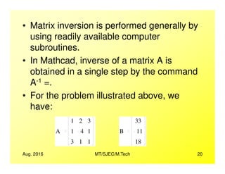
• Solution of this system by matrix inversion
method is given by:
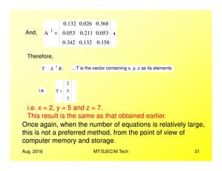
[T] = [A]-1 [B], where [A]-1 is the inverse of
matrix [A].
20. • Matrix inversion is performed generally by
using readily available computer
subroutines.
• In Mathcad, inverse of a matrix A is
obtained in a single step by the command
A-1 =.
Aug. 2016 MT/SJEC/M.Tech 20
A =.
• For the problem illustrated above, we
have:
A
1
1
3
2
4
1
3
1
1
B
33
11
18
21. And, A
1
0.132
0.053
0.342
0.026
0.211
0.132
0.368
0.053
0.158
=
Therefore,
T A
1
B. ...T is the vector containing x, y, z as its elements
2
Aug. 2016 MT/SJEC/M.Tech 21
i.e. T
2
5
7
=
i.e. x = 2, y = 5 and z = 7.
This result is the same as that obtained earlier.
Once again, when the number of equations is relatively large,
this is not a preferred method, from the point of view of
computer memory and storage.
22. (iii) Gauss–Siedel iteration method:
• Iteration methods are used when the number
of algebraic equations to be solved is relatively
large.
• Gauss-Siedel iteration (also called Liebmann
iteration) method is one of the most popular
Aug. 2016 MT/SJEC/M.Tech 22
iteration methods because of its simplicity.
• The method involves the following steps:
• (i) Solve each equation for one of the
unknowns, i.e. write each unknown in terms of
other unknowns
23. • (ii) Assume guess values for all
unknowns, and from the equations
developed in step (a), compute the
unknowns, each time using the most
recently computed values for the
unknowns in each equation
Aug. 2016 MT/SJEC/M.Tech 23
unknowns in each equation
• (iii) Repeat this procedure until the
successive values of an unknown
converge to a specified accuracy.
24. • To illustrate this procedure, let us consider the example
given below. We have a set of equations as follows:
3 x. y 3 z. 0= ....(a)
x 2 y. z 3= .... b( )
2 x. y z 2= .....(c)
Now, write each eqn. for one of the unknowns. i.e.
Aug. 2016 MT/SJEC/M.Tech 24
Now, write each eqn. for one of the unknowns. i.e.
x
y 3 z.
3
y
3 x z( )
2
z 2 2 x. y
25. • Now, assume guess values for x, y and z.
Say, x = 1, y =1 and, z = 1. These are the
‘zeroth’ iteration values.
• With these guess values, begin the
iteration and in each equation, use the
latest values of unknowns as available.
Aug. 2016 MT/SJEC/M.Tech 25
latest values of unknowns as available.
• So, after ‘first’ iteration we have:
26. x 1 y 1 z 1 ....initial guess values
x
y 3 z.
3
i.e. x 1.333= ..with y = 1, z = 1
y
3 x z( )
2
i.e. y 1.667= ....with x = 1.333, z = 1
z 2 2 x. y i.e. z 1= ...with x = 1.333, y = 1.667
Aug. 2016 MT/SJEC/M.Tech 26
Now, for the ‘second’ iteration, continue
the procedure, with the latest values of
unknowns.
We get:
27. x 1.333 y 1.667 z 1 ....next guess values from previous iteration
x
y 3 z.
3
i.e. x 0.444= ..with y =1.667, z =-1
y
3 x z( )
2
i.e. y 1.778= ....with x=-0.444, z=-1
z 2 2 x. y i.e. z 4.667= ...with x=-0.444, y=1.778
For the ‘third’ iteration, take x = -0.444, y = 1.778 and z =
-4.667, and continue. This process is programmed easily
Aug. 2016 MT/SJEC/M.Tech 27
-4.667, and continue. This process is programmed easily
in a computer and the results normally converge within
about 100 iterations.
Of course, we can also instruct the program to stop when
the difference between successive values of unknowns
converge to a pre-determined accuracy.
28. • A simple Mathcad program to perform the above iteration is shown
below. It does the iteration 100 times. Final values of x, y and z are
returned as a vector R.
R x0
1
y0
1
z0
1
xi 1
yi
3 zi
.
i 0 100..∈for
2
Aug. 2016 MT/SJEC/M.Tech 28
xi 1
3
yi 1
3 xi 1
zi
2
zi 1
2 2 xi 1
. yi 1
xi 1
yi 1
zi 1
R
2
3
1
=
And,
i.e. x = 2, y = 3 and z = -1.
29. • In the above program:
• LHS defines a vector R.
• On the RHS, there are 10 lines.
• First three lines assign the initial guess values
for x, y and z.
• Next 4 lines show the ‘ for loop’, for 100
iterations, wherein x, y and z are calculated,
Aug. 2016 MT/SJEC/M.Tech 29
iterations, wherein x, y and z are calculated,
each time using the latest available values of
unknowns.
• Next 3 lines constitute the latest values of x, y
and z which are stored as the elements of the
vector R.
30. • It is interesting to note that in the above
program, if iteration is carried out only for
5,10, 20, 50 and 100 loops (by changing
the 4th line), following are the results:
After 5 After 10 After 20 After 50 After 100
Aug. 2016 MT/SJEC/M.Tech 30
iterations
R
1.755
2.718
1.208
=
iterations
R
1.987
2.982
1.008
=
After 20
iterations
R
2
3
1
=
After 50
iterations
R
2
3
1
=
After 100
iterations
R
2
3
1
=
31. • i.e. even with only 10 iterations we are very
close to the final result. By the time 20 iterations
are over, solution has already converged to the
final result.
• It is stated that for steady state heat conduction
problems, Gauss–Siedel iteration process is
inherently stable and always converges into a
Aug. 2016 MT/SJEC/M.Tech 31
inherently stable and always converges into a
solution.
• Note: Of course, above program can be further
refined to stop when the successive values of x,
y and z differ by a pre-determined small value ε.
(say, ε = 0.001).
32. • Above program in Mathcad is shown
only to illustrate the procedure of
iterative solution.
• While actually using Mathcad, we
would use the ‘Solve block’ (which
also follows an iterative algorithm), as
Aug. 2016 MT/SJEC/M.Tech 32
also follows an iterative algorithm), as
follows:
33. x 0 y 0 z 0 ...guess values
Given
3 x. y 3 z. 0 ....(a)
x 2 y. z 3 .... b( )
2 x. y z 2 .....(c)
2
Aug. 2016 MT/SJEC/M.Tech 33
Find x y, z,( )
2
3
1
=
You may put any guess value to start with; it
makes no difference on the final result.
However, it is essential that each unknown is
assigned some guess value to start with.
34. Solution with ‘Engineering Equation
Solver (EES)’
• Above mentioned 3 equations are solved very easily
using EES, as follows:
• Enter the 3 equations in the ‘Equations Window’ as
shown.
• Press F2
Aug. 2016 MT/SJEC/M.Tech 34
• Press F2
• The equations are solved and the results appear in the
‘Solutions Window’
• A screen–shot containing both the Equations Window
and the Solutions Window is shown below:
36. Accuracy of the solutions:
• Some comments on the accuracy of finite
difference solutions are appropriate:
• We noted earlier that, accuracy improves
as the number of nodes is made larger.
• However, this would mean that a larger
number of algebraic equations have to be
Aug. 2016 MT/SJEC/M.Tech 36
number of algebraic equations have to be
solved simultaneously.
• This situation has following inherent draw
backs: the computer memory required
increases and also, more importantly, the
round off errors in successive calculations
increase since they are cumulative.
37. • Therefore, one should start with a
coarse mesh and then gradually
refine it depending upon the accuracy
of final results required.
• Note that for the normal problems
encountered in practice, a coarse
mesh generally gives results of
Aug. 2016 MT/SJEC/M.Tech 37
mesh generally gives results of
acceptable accuracy.
• Remember that, anyway, there are
uncertainties in the values of thermal
properties and heat transfer
coefficients available to the designer.
38. One-dimensional, steady state
conduction in cylindrical systems:
• We shall now develop finite difference
formulation by energy balance method:
• Consider a long, solid cylinder of radius R in
which the heat flow is only in the radial direction.
Let the rate of internal heat generation be qg
(W/m3).
Aug. 2016 MT/SJEC/M.Tech 38
g
(W/m3).
• The region from r = 0 to r = R is divided into M
sub-regions, each of thickness ∆r = R/M.
• Therefore, there are (M + 1) nodes, numbered
as 0, 1, 2,….M.
• See Fig. 8.5.
40. • Writing an energy balance for the volume
element around node ‘m’, remembering that all
heat flows are into the volume, we get:
Tm 1
Tm
∆ r
2 π. m ∆ r. ∆ r
2
. L. k.
Tm 1
Tm
∆ r
2 π. m ∆ r. ∆ r
2
. L. k.
2 π. m. ∆ r. ∆ r.( ) L. q m
. 0
Tm 1
Tm
∆ r
2 π. m ∆ r. ∆ r
2
. L. k.
Tm 1
Tm
∆ r
2 π. m ∆ r. ∆ r
2
. L. k.
2 π. m. ∆ r. ∆ r.( ) L. q m
. 0
Aug. 2016 MT/SJEC/M.Tech 40
2 2
First term in the above eqn. is the heat flowing into
node ‘m’ from node ‘(m – 1)’.
Denominator of the first term is the thermal
resistance between ‘m’ and ‘(m – 1)’;
2 2
41. • It is written in the form (L/k A) where A is
the mean area i.e. area of the plane mid-
way between nodes ‘m’ and ‘(m – 1)’.
• This form of thermal resistance ( as if for a
plane wall), is alright for the cylindrical
system when ∆r << R, which is generally
the case.
Aug. 2016 MT/SJEC/M.Tech 41
the case.
• Second term in the above eqn. is the heat
flowing into node ‘m’ from node ‘(m + 1)’.
• The third term gives the heat generated in
the elemental volume.
42. • L is the length of the cylinder and qm is the
heat gen. rate per unit volume for the
elemental volume ( = qg, generally).
• Simplifying the above equation, we get:
1
1
2 m.
Tm 1
. 2 Tm
. 1
1
2 m.
Tm 1
.
∆ r( )
2
q m
.
k
0 .....(8.32)
Aug. 2016 MT/SJEC/M.Tech 42
2 m 2 m k
Eqn. (8.32) is the finite difference eqn. for
internal nodes i.e. for nodes 1, 2, ….(M-1),
with constant thermal conductivity and
internal heat generation.
43. At the centre: i.e. at r = 0:
Writing the energy balance for the half-volume
(of thickness ∆r/2) around node ‘0’, we get:
T 1 T 0
∆ r
2 π. ∆ r
2
. L. k.
π
∆ r
2
2
. L. q 0
. 0
In the above, first term is the heat conduction rate from
node ‘1’ to node ‘0’ and the second term is the heat
Aug. 2016 MT/SJEC/M.Tech 43
node ‘1’ to node ‘0’ and the second term is the heat
generation term.
Simplifying the above equation, we get:
4 T 1 T 0
.
∆ r( )
2
q 0
.
k
0 ......(8.33)
Eqn. (8.33) gives the finite difference eqn. for the centre node ‘0’.
44. At the centre: i.e. at r = 0:
Writing the energy balance for the half-volume (of thickness ∆r/2)
around node ‘0’, we get:
T 1 T 0
∆ r
2 π. ∆ r
2
. L. k.
π
∆ r
2
2
. L. q 0
. 0
In the above, first term is the heat conduction rate from node ‘1’ to
Aug. 2016 MT/SJEC/M.Tech 44
In the above, first term is the heat conduction rate from node ‘1’ to
node ‘0’ and the second term is the heat generation term.
Simplifying the above equation, we get:
4 T 1 T 0
.
∆ r( )
2
q 0
.
k
0 ......(8.33)
Eqn. (8.33) gives the finite difference eqn. for the centre node ‘0’.
45. • At the periphery: i.e. at node ‘M’:
• Here too, finite difference equation is obtained by
applying the energy balance to the half-volume around
node ‘M’.
• Of course, the nature of equation depends on the
boundary condition.
• For convection boundary conditions, where heat transfer
from the periphery is with an ambient at temperature Ta
Aug. 2016 MT/SJEC/M.Tech 45
from the periphery is with an ambient at temperature Ta
with a heat transfer coeff. of h, energy balance around
node ‘M’, gives:
TM 1
TM
∆ r
2 π. M ∆ r. ∆ r
2
. L. k.
2 π. M ∆ r. L.( ) h. T a T M
. 2 π. M. ∆ r. ∆ r
2
. L. qM
. 0
46. • Simplifying:
1
1
T. 1
1 ∆ r h.
T. ∆ r h.
T.
∆ r( )
2
q
M
.
0 ....(8.34)
In the above eqn., first term is the heat conduction rate
from node‘(M-1)’ to node ‘M’ and the second term is the
convective heat transfer between the periphery and the
ambient, and the third term is the heat generation term.
Aug. 2016 MT/SJEC/M.Tech 46
1
1
2 M.
TM 1
. 1
1
2 M.
∆ r h.
k
TM
. ∆ r h.
k
T a
. M
2 k.
0 ....(8.34)
Eqn. (8.34) gives the finite difference eqn. for the
boundary node ‘M’, with convection conditions, constant
thermal conductivity and internal heat generation.
47. One-dimensional, steady state
conduction in spherical systems:
• Consider a solid sphere of radius R in which the
heat flow is only in the radial direction.
• Let the rate of internal heat generation be qg
(W/m3).
• The region from r = 0 to r = R is divided into M
Aug. 2016 MT/SJEC/M.Tech 47
• The region from r = 0 to r = R is divided into M
sub-regions, each of thickness ∆r = R/M.
• Therefore, there are (M + 1) nodes, numbered
as 0, 1, 2,….M.
• See Fig. 8.5.
49. • Writing an energy balance for the volume
element around node ‘m’, remembering
that all heat flows are into the volume, we
get:
Tm 1
Tm
∆ r
4 π. m ∆ r. ∆ r
2
. k.
Tm 1
Tm
∆ r
4 π. m ∆ r. ∆ r
2
. k.
4 π. m ∆ r.( )
2
. ∆ r. q m
. 0 ....(8.35)
Aug. 2016 MT/SJEC/M.Tech 49
4 π. m ∆ r. ∆ r
2
. k. 4 π. m ∆ r. ∆ r
2
. k.
First term in the above eqn. is the heat
flowing into node ‘m’ from node ‘(m – 1)’.
Denominator of the first term is the thermal
resistance between ‘m’ and ‘(m – 1)’.
50. • It is written in the form (L/k A) where A is
the mean area i.e. area of the plane mid-
way between nodes ‘m’ and ‘(m – 1)’.
• This form of thermal resistance ( as if for a
plane wall), is alright for the spherical
system when ∆r << R, which is generally
the case.
Aug. 2016 MT/SJEC/M.Tech 50
the case.
• Second term in the above eqn. is the heat
flowing into node ‘m’ from node ‘(m + 1)’.
• The third term gives the heat generated in
the elemental volume.
51. • qm is the heat gen. rate per unit volume for
the elemental volume ( = qg, generally).
• Simplifying the above equation, we get:
1
1
2 m.
2
Tm 1
Tm
. 1
1
2 m.
2
Tm 1
Tm
.
∆ r( )
2
q m
.
k
0 .....(8.36)
Aug. 2016 MT/SJEC/M.Tech 51
Eqn. (8.36) gives finite difference equations
for internal nodes, i.e. nodes 1, 2, ….(M-1).
52. • At the centre, r = 0:
• Applying the energy balance to the half-volume
around node ‘0’:
T 1 T 0
∆ r
4 π. ∆ r
2
2
. k.
4
3
π. ∆ r
2
3
. q 0
. 0
Aug. 2016 MT/SJEC/M.Tech 52
Simplifying, 6 T 1 T 0
.
∆ r( )
2
q 0
.
k
0 ......(8.37)
Eqn. (8.37) gives finite difference eqn. for the centre
i.e. node ‘0’.
53. • The nature of relation obtained will depend
upon the boundary condition i.e.
prescribed temperature, prescribed heat
flux, or convection boundary condition.
• Let us write the difference eqn. for node
For the boundary node ‘M’:
Aug. 2016 MT/SJEC/M.Tech 53
• Let us write the difference eqn. for node
“M’ when convection conditions prevail at
the boundary:
• Let there be heat transfer at the boundary
with a fluid flowing at a temperature of Ta
with a heat transfer coeff. of ‘h’.
54. • Then, writing an energy balance for the
half-volume around node ‘M’, we get:
TM 1
TM
∆ r
4 π. M ∆ r. ∆ r
2
2
. k.
4 π. M ∆ r.( )
2
h. T a T M
. 4 π. M ∆ r.( )
2
. ∆ r
2
. qM
. 0 ...(8.38)
•In the above, the first term is the heat
Aug. 2016 MT/SJEC/M.Tech 54
•In the above, the first term is the heat
conduction rate from node ‘(M-1)’ to
node ‘M’.
•The second term is the convective heat
transfer between the outer surface and
the ambient, and
55. • the third term is the heat generation term.
• qM is the heat generation rate per unit
volume at node ‘M’ ( = qg, generally).
• Simplifying the above equation, we get:
1
1
2
T. 1
1
2
∆ r h.
T. ∆ r h.
T.
∆ r( )
2
q
M
.
0 ....(8.39)
Aug. 2016 MT/SJEC/M.Tech 55
1
1
2 M.
TM 1
. 1
1
2 M.
∆ r h.
k
TM
. ∆ r h.
k
T a
. M
2 k.
0 ....(8.39)
Eqn. (8.39) gives the difference eqn. for
the boundary node ‘M’ when convection
conditions prevail at the boundary.
63. Two-dimensional, steady state
conduction in cartesian coordinates:
• Examples where temperature gradients are
significant in more than one direction: large
chimneys and L–shaped bars etc.
• Consider a two-dimensional system in which
Aug. 2016 MT/SJEC/M.Tech 63
• Consider a two-dimensional system in which
temperature gradients are significant in the x
and y directions.
• Let the x-y plane be subdivided into rectangular
mesh of nodes, with spacing of ∆x and ∆y in x
and y directions respectively.
64. Two-dimensional, steady state
conduction in cartesian coordinates:
• Then, the nodes are numbered with a
double subscript notation. i.e. a typical
node, T m,n is the node with a x-coordinate
of (m.∆x) and y-coordinate of (n.∆y).
Aug. 2016 MT/SJEC/M.Tech 64
of (m.∆x) and y-coordinate of (n.∆y).
• Node count is m = 0, 1, ..M in the x
direction and n = 0, 1,….N in the y
direction. See Fig. 8.6.
65. Aug. 2016 MT/SJEC/M.Tech 65
• We see that there are basically three types of nodes:
internal nodes, surface nodes, and corner nodes,
marked 1, 2 and 3 respectively in the fig. 8.6(a).
66. • Difference equations for different nodes
are written by making an energy balance
for the elemental volume around the node
in question, with all the heat flow lines
going into the volume.
• Elemental volumes for the internal node,
Aug. 2016 MT/SJEC/M.Tech 66
• Elemental volumes for the internal node,
surface node and corner nodes are shown
by dotted lines around the nodes, in the
above fig.
67. • Difference equations for internal
nodes:
• Consider a typical internal node, Tm,n in
the x-y plane, with unit depth
perpendicular to the plane of paper, as
shown in Fig. 8.6(b).
• It is surrounded by 4 nodes: T , T ,
Aug. 2016 MT/SJEC/M.Tech 67
• It is surrounded by 4 nodes: Tm-1,n , Tm,n+1 ,
Tm+1,n , and Tm,n-1.
• Let us make an energy balance on the
elemental volume surrounding the node
Tm,n .
68. • It is observed that heat flows into the node
from all the four directions, i.e. left, right,
up and down.
• In addition, let there be heat generation in
the volume at a rate of (∆V.qg) , W, where
qg , (W/m3), is the uniform volumetric heat
generation rate in the system.
Aug. 2016 MT/SJEC/M.Tech 68
g
generation rate in the system.
• Writing the energy balance, in steady
state:
69. Q left Q right Q up Q down ∆ V q g
. 0 .....(8.40)
i.e.
k ∆ y.
Tm 1 n,
Tm n,
∆ x
. k ∆ y.
Tm 1 n,
Tm n,
∆ x
. k ∆ x.
Tm n 1,
Tm n,
∆ y
. k ∆ x.
Tm n 1,
Tm n,
∆ y
. q g ∆ x. ∆ y. 0
Simplifying, we get,
Aug. 2016 MT/SJEC/M.Tech 69
Tm 1 n,
2 Tm n,
. Tm 1 n,
∆ x( )
2
Tm n 1,
2 Tm n,
. Tm n 1,
∆ y( )
2
q g
k
0 ....(8.41)
Eqn. (8.41) gives the difference eqn. for internal nodes,
i.e. for m = 1,2,…(M-1), and n = 1,2,….(N-1).
70. • Now, generally a square mesh is used i.e. ∆x =
∆y = (∆x , say). Then, the eqn.(8.41) simplifies
to:
Tm 1 n,
Tm 1 n,
Tm n 1,
Tm n 1,
4 Tm n,
.
q g ∆x( )
2.
k
0 .....(8.42)
Eqn.(8.42) is the finite difference eqn. for the
internal nodes, with ∆x = ∆y .
Aug. 2016 MT/SJEC/M.Tech 70
internal nodes, with ∆x = ∆y .
When there is no heat generation in the body,
the difference eqn. for the node reduces to:
Tm n,
Tm 1 n,
Tm 1 n,
Tm n 1,
Tm n 1,
4
.....(8.43)
71. • i.e., when there is no heat generation, and
a square mesh is used in the analysis,
temperature of an internal node is given as
the arithmetic average of the surrounding
four temperatures.
• Difference equations for boundary nodes:
• Boundary nodes may be on the surface or
on the corners.
Aug. 2016 MT/SJEC/M.Tech 71
on the corners.
• Difference equations are developed for
boundary nodes in a similar manner as for
interior nodes, i.e. by making an energy
balance on the elemental volume
surrounding the node.
72. • In Fig. 8.6(a), we can see that the surface
node 2 is surrounded by a half-volume and
the corner node 3 has a quarter volume
attached to it.
• Exact form of the difference equation will
depend upon the boundary conditions i.e.
Aug. 2016 MT/SJEC/M.Tech 72
depend upon the boundary conditions i.e.
prescribed temperature, prescribed heat
flux, insulated, convection or radiation
boundary conditions.
• Fig. (8.7) shows some common boundary
conditions encountered in practice.
74. • Example: Develop finite difference
equations for an interior corner node with
convection conditions, using the energy
balance method. See Fig. 8.7(a).
• As shown in the fig., elemental volume
around the node is ¾ of full volume.
Aug. 2016 MT/SJEC/M.Tech 74
around the node is ¾ of full volume.
Writing an energy balance for this volume,
we apply eqn. (8.40):
Q left Q right Q up Q down ∆V q g
. 0 .....(8.40)
75. i.e.
k ∆y.
Tm 1 n,
Tm n,
∆x
. k
∆y
2
.
Tm 1 n,
Tm n,
∆x
. k ∆x.
Tm n 1,
Tm n,
∆y
. k
∆x
2
.
Tm n 1,
Tm n,
∆y
. q g
3
4
∆x. ∆y.. 0
Remembering that ∆x = ∆y =(∆x, say), we get on
simplification,
Aug. 2016 MT/SJEC/M.Tech 75
Tm n 1,
2 Tm 1 n,
. 2 Tm n 1,
. Tm 1 n,
6
2 h. ∆x.
k
Tm n,
. 3
2
∆x( )
2
.
q g
k
. 2 h. ∆x.
k
T a
. 0
And, if there is no internal heat generation,
Tm n 1,
2 Tm 1 n,
. 2 Tm n 1,
. Tm 1 n,
6
2 h. ∆x.
k
Tm n,
. 2 h. ∆x.
k
T a
. 0 ....(8.44)
76. Summary of steady state, finite difference
equations for different boundary conditions:
(q = heat flux, h = conv. heat tr. coeff., k = thermal cond.,
no int. heat gen., and ∆∆∆∆x = ∆∆∆∆y)
(1) Node at an internal corner with convection (Fig. (8.7,a):
Tm n 1,
2 Tm 1 n,
. 2 Tm n 1,
. Tm 1 n,
6
2 h. ∆x.
k
Tm n,
. 2 h. ∆x.
k
T a
. 0 ....(8.44)
--------------------------------------------------------------------------------------------------
Aug. 2016 MT/SJEC/M.Tech 76
(2) Node at a plane surface with convection (Fig. (8.7,b):
2 Tm 1 n,
. Tm n 1,
Tm n 1,
2 h. ∆x.
k
T a
. 2
h ∆x.
k
2. Tm n,
. 0 ....(8.45)
(3) Node at an external corner with convection (Fig. (8.7,c):
Tm n 1,
Tm 1 n,
2 h. ∆x.
k
T a
. 2
h ∆x.
k
1. Tm n,
. 0 ....(8.46)
77. (4) Node at a plane surface with uniform heat flux (Fig. (8.7,d):
2 Tm 1 n,
. Tm n 1,
Tm n 1,
2 q. ∆x.
k
4 Tm n,
. 0 ....(8.47)
Note: In eqns.(8.42) and (8.44), put h = 0 or q = 0, to get difference
equations for an insulated surface or a surface with thermal symmetry.
--------------------------------------------------------------------------------------------------
Aug. 2016 MT/SJEC/M.Tech 77
78. • Example 8.8: For the two-dimensional region shown in Fig.
Ex. 8.8, with constant k ( = 20 W/(m.C)) and no internal heat
generation, and with the indicated boundary conditions,
formulate the finite difference equations and solve for unknown
temperatures. Use ∆∆∆∆x = ∆∆∆∆y = 1 cm.
Aug. 2016 MT/SJEC/M.Tech 78
79. Data:
∆ x 0.01 m
∆ y 0.01 m
T a 20 C.....ambient temp.
h 50 W/(m2.C).....heat transfer coeff.
k 20 W/(m.C)....thermal cond.
Nodes are represented by numbers 1, 2,.....7. Elemental volume
Aug. 2016 MT/SJEC/M.Tech 79
Nodes are represented by numbers 1, 2,.....7. Elemental volume
pertinent to each node is also marked around it and numbered a, b,....r.
For node 1:
Elemental volume to be considered is 1/4 volume,
1-a-b-c-1.
80. • For this elemental volume, considering unit depth, heat transfers
into the volume are:
• From left surface, there is no heat transfer, since it is insulated.
i.e. Q left 0
From top, i.e surface 1-a: there is convection:
i.e. Q top h
∆ x
2
1.. T a T 1
.
From right, there is conduction from node 3 through surface a-b:
Aug. 2016 MT/SJEC/M.Tech 80
From right, there is conduction from node 3 through surface a-b:
i.e. Q right k
∆ y
2
1..
T 3 T 1
∆ x
.
From down, there is conduction from node 2 through surface b-c:
i.e. Q down k
∆ x
2
1..
T 2 T 1
∆ y
.
81. • There is no heat generation term in this problem.
• So, heat balance on the elemental volume for node 1 gives:
h
∆ x
2
1.. T a T 1
. k
∆ y
2
1..
T 3 T 1
∆ x
. k
∆ x
2
1..
T 2 T 1
∆ y
. 0
i.e. 0.25 T a T 1
. 10 T 3 T 1
. 10 T 2 T 1
. 0 ....(a)
Eqn. (a) is the difference eqn. for node 1.
Aug. 2016 MT/SJEC/M.Tech 81
For node 2:
Here, elemental volume to be considered is 1/2 volume, c-b-e-r. and,
energy balance can be written as we did for node 1.
However, since the surface is insulated, it is easier to use the mirror
image concept and consider the node 2 as an internal node.
So, to the left of node 2, we have T4, mirror image of temp. of node 4.
Then, considering 2 as internal node, we get difference eqn for node 2:
82. • For node 3:
• This is a corner node with convection . Elemental volume to be
considered is 1/4 volume, a-3-d-b.
• We can directly apply eqn. (8.46), viz.
T 4 T 1 T 4 150 4 T 2
. 0 .....(b)
Tm n 1,
Tm 1 n,
2 h. ∆x.
k
T a
. 2
h ∆x.
k
1. Tm n,
. 0 ....(8.46)
Aug. 2016 MT/SJEC/M.Tech 82
k k
i.e. T 4 T 1 0.05 T a
. 2.05 T 3
. 0 ....(c)
For node 4:
This is an internal corner node with convection . Elemental volume to be
considered is 3/4 volume, g-f-e-b-d-4.
Again, we can directly apply eqn. (8.44), viz.
83. • For node 5:
• This is a surface node with convection . Elemental volume to be
considered is 1/2 volume, g-f-i-h-g.
Tm n 1,
2 Tm 1 n,
. 2 Tm n 1,
. Tm 1 n,
6
2 h. ∆x.
k
Tm n,
. 2 h. ∆x.
k
T a
. 0 ....(8.44)
i.e. 150 2 T 2
. 2 T 3
. T 5 6.05 T 4
. 0.05 T a
. 0 .....(d)
Eqn.(d) is the difference eqn. for node 4.
Aug. 2016 MT/SJEC/M.Tech 83
• Again, we can directly apply eqn. (8.45), viz.
2 Tm 1 n,
. Tm n 1,
Tm n 1,
2 h. ∆x.
k
T a
. 2
h ∆x.
k
2. Tm n,
. 0 ....(8.45)
Remembering that eqn. (8.45) was developed for a vertical surface,
and in the present case, we are dealing with a horizontal surface, we
can write:
2 150. T 4 T 6 0.05 T a
. 4.05 T 5
. 0 ....(e)
84. • For node 7:
• This is a corner node with conduction from left, convection on the
top, insulated on the right, and conduction from down. Elemental
volume to be considered is 1/4 volume, k-7-p-j.
• Writing the energy balance:
For node 6:
This is identical to node 5. So, we get:
2 150. T 5 T 7 0.05 T a
. 4.05 T 6
. 0 ....(f)
Aug. 2016 MT/SJEC/M.Tech 84
• Writing the energy balance:
k
∆ y
2
1..
T 6 T 7
∆ x
. h
∆ x
2
1.. T a T 7
. 0 k
∆ x
2
1..
150 T 7
∆ y
. 0
i.e. 10 T 6 T 7
. 0.25 T a T 7
. 10 150 T 7
. 0 ....(g)
Temperatures at nodes 1 to 7 are obtained by simultaneously solving 7
equations (a) to (g).
85. • We use 'solve block'of Mathcad to solve this set of equations.
• Start with guess values for all unknown temperatures and
immediately below 'Given', type the constraint equations. Then, the
command 'Find(T1,...T7)'gives the temperatures immediately:
...guess values of
temperatures
T 1 50 T 2 50 T 3 50 T 4 50 T 5 50 T 6 50 T 7 50
Given
Aug. 2016 MT/SJEC/M.Tech 85
0.25 T a T 1
. 10 T 3 T 1
. 10 T 2 T 1
. 0 ....(a)
T 4 T 1 T 4 150 4 T 2
. 0 .....(b)
T 4 T 1 0.05 T a
. 2.05 T 3
. 0 ....(c)
150 2 T 2
. 2 T 3
. T 5 6.05 T 4
. 0.05 T a
. 0 .....(d)
2 150. T 4 T 6 0.05 T a
. 4.05 T 5
. 0 ....(e)
86. 2 150. T 5 T 7 0.05 T a
. 4.05 T 6
. 0 ....(f)
10 T 6 T 7
. 0.25 T a T 7
. 10 150 T 7
. 0 ....(g)
Temp Find T 1 T 2, T 3, T 4, T 5, T 6, T 7, ....node temps. are stored in vector 'Temp'.
i.e. Temp
138.552
142.929
137.139
141.582=
T1
138.552 C
T2
142.929 C
T 137.139 C
Aug. 2016 MT/SJEC/M.Tech 86
i.e. Temp 141.582
145.437
146.438
146.636
=
i.e. The node temperatures are:
T3
137.139 C
T4
141.582 C
T5
145.437 C
T6
146.438 C
T7
146.636 C
87. • Example 8.9: A very long bar of square cross-section
has its four sides held at constant temperatures as
shown in Fig. Ex. 8.9. Determine the temperatures at
the internal nodes. Compare the results with
analytical solution.
Aug. 2016 MT/SJEC/M.Tech 87
88. • There are 9 internal nodes. Difference eqns. for these nodes are
obtained by applying eqn.(8.42), viz.
Tm 1 n,
Tm 1 n,
Tm n 1,
Tm n 1,
4 Tm n,
.
q g ∆ x( )
2.
k
0 .....(8.42)
In the present case, there is no internal heat generation. So, the last
term of the above eqn. will be zero. Therefore, we get:
Node 1: 150 200 T 2 T 4 4 T 1
. 0 .....(a)
Node 2: T 1 200 T 3 T 5 4 T 2
. 0 .....(b)
Aug. 2016 MT/SJEC/M.Tech 88
1 3 5 2
Node 3: T 2 200 150 T 6 4 T 3
. 0 .....(c)
Node 4: 150 T 1 T 5 T 7 4 T 4
. 0 .....(d)
Node 5: T 4 T 2 T 6 T 8 4 T 5
. 0 .....(e)
Node 6: T 5 T 3 150 T 9 4 T 6
. 0 .....(f)
Node 7: 150 T 4 T 8 150 4 T 7
. 0 .....(g)
Node 8: T 7 T 5 T 9 150 4 T 8
. 0 .....(h)
Node 9: T 8 T 6 150 150 4 T 9
. 0 .....(i)
89. • By solving these eqns. simultaneously, we get the temperatures at
nodes 1 to 9.
• We use 'solve block'of Mathcad to solve this set of equations.
• Start with guess values for all unknown temperatures and immediately
below 'Given', type the constraint equations. Then, the command
'Find(T1,...T9)'gives the temperatures immediately:
T 1 50 T 2 50 T 3 50 T 4 50 T 5 50
...guess values of
temperaturesT 6 50 T 7 50 T 8 50 T 9 50
Given
150 200 T 2 T 4 4 T 1
. 0 .....(a)
Aug. 2016 MT/SJEC/M.Tech 89
150 200 T 2 T 4 4 T 1
. 0 .....(a)
T 1 200 T 3 T 5 4 T 2
. 0 .....(b)
T 2 200 150 T 6 4 T 3
. 0 .....(c)
150 T 1 T 5 T 7 4 T 4
. 0 .....(d)
T 4 T 2 T 6 T 8 4 T 5
. 0 .....(e)
T 5 T 3 150 T 9 4 T 6
. 0 .....(f)
150 T 4 T 8 150 4 T 7
. 0 .....(g)
T 7 T 5 T 9 150 4 T 8
. 0 .....(h)
T 8 T 6 150 150 4 T 9
. 0 .....(i)
90. Temp Find T 1 T 2, T 3, T 4, T 5, T 6, T 7, T 8, T 9, ....node temps. are stored in vector 'Temp'.
i.e. Temp
171.429
176.339
171.429
159.375
162.5
159.375
153.571
154.911
153.571
=
T1
171.429 C
T2
176.339 C
T3
171.429 C
Aug. 2016 MT/SJEC/M.Tech 90
153.571
i.e. The node temperatures are:
T4
159.375 C
T5
162.5 C
T6
159.375 C
T7
153.571 C
T8
154.911 C
T9
153.571 C
91. • Comparison with analytical solution:
• Analytical solution for this problem is a little complicated and is given
in terms of an infinite series, as follows:
θ θ c
2
π
.
1
∞
n
1( )
n 1
1
n
sinh n π. y
L
.
sinh n π. W
L
.
. sin n π. x
L
..
=
.
Nomenclature for the above eqn. for the present problem is as follows:
Aug. 2016 MT/SJEC/M.Tech 91
Nomenclature for the above eqn. for the present problem is as follows:
θ T 150 ....T = temp. at the desired point; 150 C is the const. temp. on three sides
θ c 200 150 ..temp. difference between the temp. of fourth side and the const. temp.
of three sides.
n...no. of terms considered in the infinite series
x, y ....coordinates of the point where temp. is desired
L 2 m...length along x-axis
W 2 m....length along y-axis
92. • Above eqn. is solved very easily in Mathcad:
• Let us re-define as a function of (x, y), and consider
only 6 terms of the infinite series (n = 6) as shown below,
for convenience:
θ x y,( ) θ c
2
π
.
1
6
n
1( )
n 1
1
n
sinh n π. y
L
.
sinh n π. W
L
.
. sin n π. x
L
..
=
. .(A)....define θ as a
function of x and y
Aug. 2016 MT/SJEC/M.Tech 92
L
Now, substitute (x,y) corresponding to different
nodes and get the analytical temps. at those nodes
immediately:
94. • We make following important
observations:
• (i) Even with a crude mesh of 4 x 4, we get
values of temperatures at the nodes very
close to the analytical results.
• (ii) Note that the analytical relation to find
the temp. at any point is very complicated,
Aug. 2016 MT/SJEC/M.Tech 94
the temp. at any point is very complicated,
and to solve it without a computer is rather
laborious and time consuming. But, with
Mathcad, even this analytical solution is
easy to perform.
95. • (iii) Numerical method of formulating
difference eqns. by energy balance
method is easy and straight forward, only
labor being in solving the set of
simultaneous equations. But, with
Mathcad, this is also very easy.
Aug. 2016 MT/SJEC/M.Tech 95