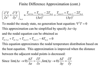
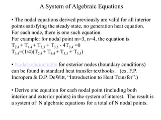
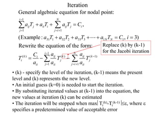
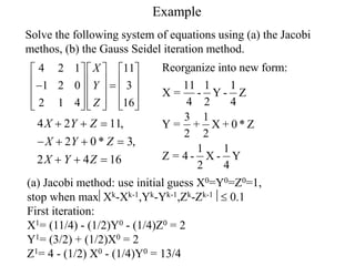
This document summarizes the finite difference method for numerically solving heat transfer problems. The method involves establishing a nodal network to discretize the domain, deriving finite difference approximations of the governing heat equation at each node, developing a system of simultaneous algebraic equations relating all nodal temperatures, and solving the system of equations using numerical techniques like matrix inversion or iterative methods. Examples are provided to illustrate the finite difference approximations, formation of the algebraic system, and solution via the Jacobi and Gauss-Seidel iteration methods.

1. Numerical Methods
Due to the increasing complexities encountered in the development
of modern technology, analytical solutions usually are not available.
For these problems, numerical solutions obtained using high-speed
computer are very useful, especially when the geometry of the object
of interest is irregular, or the boundary conditions are nonlinear. In
numerical analysis, two different approaches are commonly used:
the finite difference and the finite element methods. In heat transfer
problems, the finite difference method is used more often and will be
discussed here. The finite difference method involves:
 Establish nodal networks
 Derive finite difference approximations for the governing
equation at both interior and exterior nodal points
 Develop a system of simultaneous algebraic nodal equations
 Solve the system of equations using numerical schemes

2. The Nodal Networks
The basic idea is to subdivide the area of interest into sub-volumes
with the distance between adjacent nodes by Dx and Dy as shown.
If the distance between points is small enough, the differential
equation can be approximated locally by a set of finite difference
equations. Each node now represents a small region where the
nodal temperature is a measure of the average temperature of the
region.
Example:
m,n
m,n+1
m,n-1
m+1, n
m-1,n
Dy
Dx
m-½,n
intermediate points
m+½,n
x=mDx, y=nDy

3. Finite Difference Approximation
2
P
2
1
Heat Diffusion Equation: ,
k
where = is the thermal diffusivity
C
No generation and steady state: q=0 and 0, 0
t
First, approximated the first order differentiation
at intermediate
q T
T
k t
V
T




  


   

1, ,
( 1/ 2, ) ( 1/ 2, )
, 1,
( 1/ 2, ) ( 1/ 2, )
points (m+1/2,n) & (m-1/2,n)
T
x
T
x
m n m n
m n m n
m n m n
m n m n
T T
T
x x
T T
T
x x

 

 

 D
 
 D D

 D
 
 D D

4. Finite Difference Approximation (cont.)
2
1/ 2, 1/ 2,
2
,
2
1, 1, ,
2 2
,
2
Next, approximate the second order differentiation at m,n
/ /
2
( )
Similarly, the approximation can be applied to
the other dimension y
m n m n
m n
m n m n m n
m n
T x T x
T
x x
T T T
T
x x
T
 
 
    


 D
 


 D


, 1 , 1 ,
2 2
,
2
( )
m n m n m n
m n
T T T
y y
 
 

D

5. Finite Difference Approximation (cont.)
2 2
1, 1, , , 1 , 1 ,
2 2 2 2
,
2
2 2
( ) ( )
To model the steady state, no generation heat equation: 0
This approximation can be simplified by specify x= y
and the nodal
m n m n m n m n m n m n
m n
T T T T T T
T T
x y x y
T
   
   
 
 
  
 
  D D
 
 
D D
1, 1, , 1 , 1 ,
equation can be obtained as
4 0
This equation approximates the nodal temperature distribution based on
the heat equation. This approximation is improved when the distance
m n m n m n m n m n
T T T T T
   
    
between the adjacent nodal points is decreased:
Since lim( 0) ,lim( 0)
T T T T
x y
x x y y
D  D 
D   D  
D  D 

6. A System of Algebraic Equations
• The nodal equations derived previously are valid for all interior
points satisfying the steady state, no generation heat equation.
For each node, there is one such equation.
For example: for nodal point m=3, n=4, the equation is
T2,4 + T4,4 + T3,3 + T3,5 - 4T3,4 =0
T3,4=(1/4)(T2,4 + T4,4 + T3,3 + T3,5)
• Nodal relation table for exterior nodes (boundary conditions)
can be found in standard heat transfer textbooks. (ex. F.P.
Incropera & D.P. DeWitt, “Introduction to Heat Transfer”.)
• Derive one equation for each nodal point (including both
interior and exterior points) in the system of interest. The result is
a system of N algebraic equations for a total of N nodal points.

7. Matrix Form
11 1 12 2 1 1
21 1 22 2 2 2
1 1 2 2
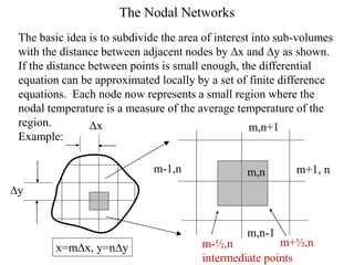
The system of equations:
N N
N N
N N NN N N
a T a T a T C
a T a T a T C
a T a T a T C
   
   
   
A total of N algebraic equations for the N nodal points and the
system can be expressed as a matrix formulation: [A][T]=[C]
11 12 1 1 1
21 22 2 2 2
1 2
= , ,
N
N
N N NN N N
a a a T C
a a a T C
where A T C
a a a T C
     
     
     
 
     
     
     

8. Numerical Solutions
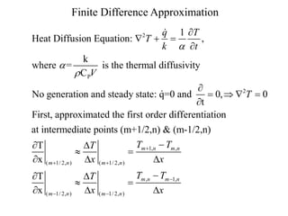
Matrix form: [A][T]=[C].
From linear algebra: [A]-1[A][T]=[A]-1[C], [T]=[A]-1[C]
where [A]-1 is the inverse of matrix [A]. [T] is the solution
vector.
• Matrix inversion requires cumbersome numerical computations
and is not efficient if the order of the matrix is high (>10)
• Gauss elimination method and other matrix solvers are usually
available in many numerical solution package. For example,
“Numerical Recipes” by Cambridge University Press or their web
source at www.nr.com.
• For high order matrix, iterative methods are usually more
efficient. The famous Jacobi & Gauss-Seidel iteration methods
will be introduced in the following.

9. Iteration
1
1 1
31 1 32 2 33 3 1 1
1
( ) ( ) ( 1)
1
General algebraic equation for nodal point:
,
(Example : , 3)
Rewrite the equation of the form:
i N
ij j ii i ij j i
j j i
N N
i
ij ij
k k k
i
i j j
j j i
ii ii ii
a T a T a T C
a T a T a T a T C i
a a
C
T T T
a a a

  


 
  
     
  
 
 1
N


• (k) - specify the level of the iteration, (k-1) means the present
level and (k) represents the new level.
• An initial guess (k=0) is needed to start the iteration.
• By substituting iterated values at (k-1) into the equation, the
new values at iteration (k) can be estimated
• The iteration will be stopped when maxTi
(k)-Ti
(k-1), where 
specifies a predetermined value of acceptable error
Replace (k) by (k-1)
for the Jacobi iteration

10. Example
Solve the following system of equations using (a) the Jacobi
methos, (b) the Gauss Seidel iteration method.
4 2 11
2 0 3
2 4 16
X Y Z
X Y Z
X Y Z
  
   
  
,
* ,
(a) Jacobi method: use initial guess X0=Y0=Z0=1,
stop when maxXk-Xk-1,Yk-Yk-1,Zk-Zk-1  0.1
First iteration:
X1= (11/4) - (1/2)Y0 - (1/4)Z0 = 2
Y1= (3/2) + (1/2)X0 = 2
Z1= 4 - (1/2) X0 - (1/4)Y0 = 13/4
Reorganize into new form:
X =
11
4
-
1
2
Y -
1
4
Z
Y =
3
2
+
1
2
X + 0 * Z
Z = 4 -
1
2
X -
1
4
Y
4 2 1 11
1 2 0 3
2 1 4 16
X
Y
Z
     
     
 
     
     
     

11. Example (cont.)
Second iteration: use the iterated values X1=2, Y1=2, Z1=13/4
X2 = (11/4) - (1/2)Y1 - (1/4)Z1 = 15/16
Y2 = (3/2) + (1/2)X1 = 5/2
Z2 = 4 - (1/2) X1 - (1/4)Y1 = 5/2
Final solution [1.014, 2.02, 2.996]
Exact solution [1, 2, 3]
5 4 5 4 5 4
Converging Process:
13 15 5 5 7 63 93 133 31 393
[1,1,1], 2,2, , , , , , , , , ,
4 16 2 2 8 32 32 128 16 128
519 517 767
, , . Stop the iteration when
512 256 256
max , , 0.1
X X Y Y Z Z
       
       
       
 
 
 
   

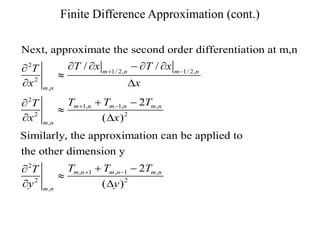
12. Example (cont.)
(b) Gauss-Seidel iteration: Substitute the iterated values into the
iterative process immediately after they are computed.
0 0 0
1 0 0
1 1
1 1 1
Use initial guess X 1
11 1 1 3 1 1 1
, , 4
4 2 4 2 2 2 4
11 1 1
First iteration: X = ( ) ( ) 2
4 2 4
3 1 3 1 5
(2)
2 2 2 2 2
1 1 1 1 5 19
4 4 (2)
2 4 2 4 2 8
5 19
Converging process: [1,1,1], 2, ,
2 8
Y Z
X Y Z Y X Z X Y
Y Z
Y X
Z X Y
  
       
  
    
 
      
 
 


29 125 783 1033 4095 24541
, , , , , ,
32 64 256 1024 2048 8192
The iterated solution [1.009, 1.9995, 2.996] and it converges faster
    
     
    
Immediate substitution