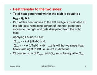
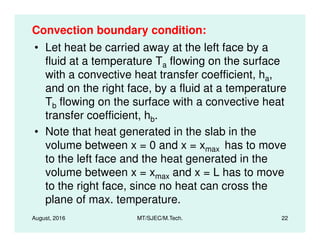
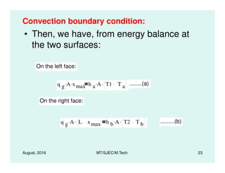
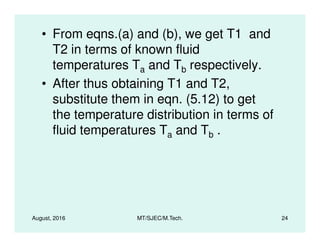
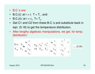
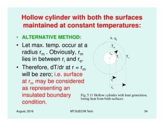
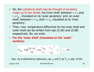
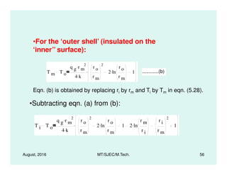
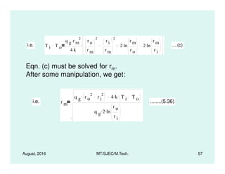
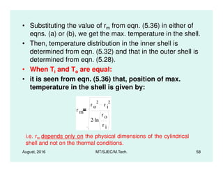
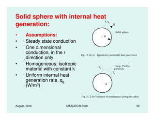
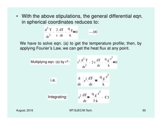
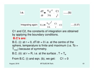
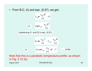
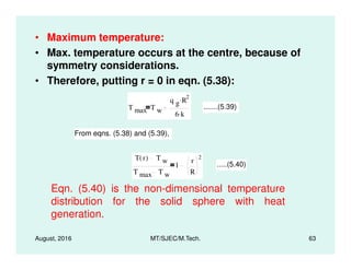
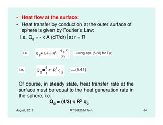
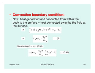
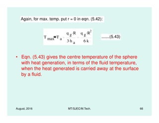
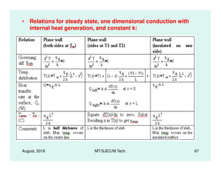
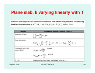
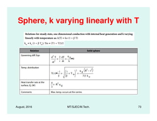
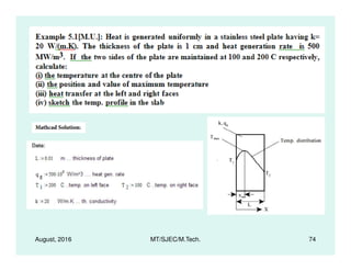
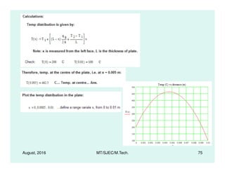
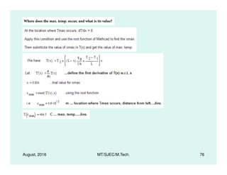
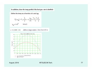
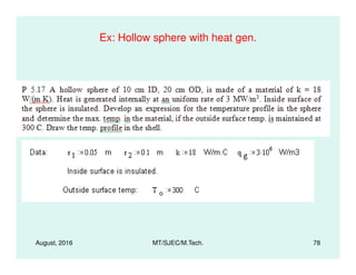
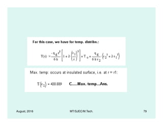
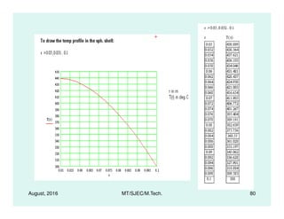
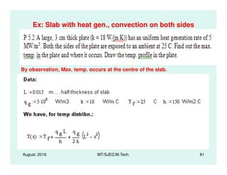
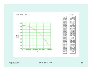
One dim, steady-state, heat conduction_with_heat_generation

Lectures on Heat Transfer --
One-Dimensional, Steady-State
Heat Conduction with Heat
Generation
by
Dr. M. ThirumaleshwarDr. M. Thirumaleshwar
formerly:
Professor, Dept. of Mechanical Engineering,
St. Joseph Engg. College, Vamanjoor,
Mangalore

Preface
• This file contains slides on One-
dimensional, steady-state heat
conduction with heat generation.
• The slides were prepared while teaching• The slides were prepared while teaching
Heat Transfer course to the M.Tech.
students in Mechanical Engineering Dept.
of St. Joseph Engineering College,
Vamanjoor, Mangalore, India, during Sept.
– Dec. 2010.
August, 2016 2MT/SJEC/M.Tech.

• It is hoped that these Slides will be useful
to teachers, students, researchers and
professionals working in this field.
• For students, it should be particularly
useful to study, quickly review the subject,useful to study, quickly review the subject,
and to prepare for the examinations.
•
August, 2016 3MT/SJEC/M.Tech.

References
• 1. M. Thirumaleshwar: Fundamentals of Heat &
Mass Transfer, Pearson Edu., 2006
• https://books.google.co.in/books?id=b2238B-
AsqcC&printsec=frontcover&source=gbs_atb#v=onepage&q&f=false
• 2. Cengel Y. A. Heat Transfer: A Practical
Approach, 2nd Ed. McGraw Hill Co., 2003
August, 2016 MT/SJEC/M.Tech. 4
Approach, 2nd Ed. McGraw Hill Co., 2003
• 3. Cengel, Y. A. and Ghajar, A. J., Heat and
Mass Transfer - Fundamentals and Applications,
5th Ed., McGraw-Hill, New York, NY, 2014.

References… contd.
• 4. Incropera , Dewitt, Bergman, Lavine:
Fundamentals of Heat and Mass Transfer, 6th
Ed., Wiley Intl.
• 5. M. Thirumaleshwar: Software Solutions to• 5. M. Thirumaleshwar: Software Solutions to
Problems on Heat Transfer – CONDUCTION-
Part-II, Bookboon, 2013
• http://bookboon.com/en/software-solutions-problems-on-heat-
transfer-cii-ebook

One-Dimensional, Steady-State
Heat Conduction with Heat
Generation
• Examples - Plane slab – different BC’s -
Cylindrical Systems – Solid cylinder – hollow
cylinder – different BC’s – Sphere with heat
cylinder – different BC’s – Sphere with heat
generation- k varying linearly with T

Examples of situations with internal
heat generation are:
• Joule heating in an electrical conductor
due to the flow of current in it
• Energy generation in a nuclear fuel rod
due to absorption of neutrons
• Exothermic chemical reaction within a
system (e.g. combustion), liberating heat
at a given rate throughout the system

Examples (contd.)
• Heat liberated in ‘shielding’ used in
Nuclear reactors due to absorption of
electromagnetic radiation such as
gamma rays
• Curing of concrete
• Curing of concrete
• Magnetization of iron
• Ripening of fruits and in biological decay
processes

Plane slab with uniform internal
heat generation:
• We shall consider three cases of
boundary conditions:
• 1. Both the sides of the slab are at the
same temperature
same temperature
• 2. Two sides of the slab are at different
temperatures, and
• 3. One of the sides is insulated

Plane slab with uniform internal heat
generation- both the sides at the same
temperature:
• Assumptions:
• One dimensional conduction i.e. thickness L is small
compared to the dimensions in the y and z directions
• Steady state conduction i.e. temperature at any point
within the slab does not change with time; of course,
temperatures at different points within the slab will be
within the slab does not change with time; of course,
temperatures at different points within the slab will be
different.
• Uniform internal heat generation rate, qg (W/m3)
• Material of the slab is homogeneous (i.e. constant
density) and isotropic (i.e. value of k is same in all
directions).

generation- both the sides at the same
temperature:
k, qg
Tw
To = Tmax
Tw
Temp. distribution-(parabolic)
X
Fig.5.1 Plane slab with internal heat
generation - both sides at the same temp.
LL

• For the above mentioned stipulations, governing eqn. in
cartesian coordinates reduces to:
d
2
T
dx
2
q g
k
0 ....(5.1)
Solution of eqn. (5.1) gives the temperature profile and then, by
using Fourier’s equation we get the heat flux at any point.
B.C’s:
B.C’s:
(i) at x = 0, dT/dx = 0, since temperature is maximum at the centre line.
(ii) at x = ± L, T = Tw
Integrating eqn. (5.1) once,
dT
dx
q g x.
k
C1 .....(a)

• Integrating again,
T
q g x
2.
2 k.
C1 x. C2 ....(5.2)
Applying B.C (i) to eqn.(a): C1 = 0
Applying B.C. (ii) to eqn. (5.2): T w
q g L
2.
2 k.
C2
2.
C2 T w
q g L
2.
2 k.i.e.
Substituting for C1 and C2 in eqn. (5.2):
T x( )
q g x
2.
2 k.
T w
q g L
2.
2 k.
i.e. T x( ) T w
q g
2 k.
L
2
x
2. ....(5.3) where L is half thickness of the
slab. (Remember this.)

• Also, by observation, T = Tmax at x = 0. (You can show
this easily by differentiating eqn. (5.3) w.r.t x and
equating to zero.)
• Then, putting x = 0 in eqn. (5.3):
T max T w
q g L
2.
2 k.
......(5.4)
Then, from eqns. (5.3) and (5.4), we get:
T T w
T max T w
L
2
x
2
L
2
1
x
L
2
....(5.5)
Eqn. (5.5) gives the non-dimensional temperature
distribution in a slab of half-thickness L, with heat
generation.
Note that the temperature distribution is parabolic, as shown in
Fig. 5.1.

Convection boundary condition:
• In many practical applications, heat is carried
away at the boundaries by a fluid at a
temperature Tf flowing on the surface with a
convective heat transfer coefficient, h. (e.g.
current carrying conductor cooled by ambient air
or nuclear fuel rod cooled by a liquid metal
or nuclear fuel rod cooled by a liquid metal
coolant).
• Then, by an energy balance at the surface:
• heat conducted from within the body to the
surface = the heat convected away by the fluid
at the surface.

• If A is the surface area of the slab (normal
to the direction of heat flow), we have,
from energy balance at the surface:
q g A. L. h A. T w T f
.
q g A. L. h A. T w T f
.
i.e. T w T f
q g L.
h
.....(5.6)

• Substituting eqn. (5.6) in eqn. (5.3),
T x( ) T f
q g L.
h
q g
2 k.
L
2
x
2. ......(5.7)
Eqn. (5.7) gives temperature distribution in a slab with heat
generation, in terms of the fluid temperature, Tf .
Remember, again, that L is half-thickness of the slab.
Heat transfer:
Heat transfer:
By observation, we know that the heat transfer rate from
either of the surfaces must be equal to half of the total
heat generated within the slab, for the B.C. of Tw being
the same at both the surfaces.
i.e. Q = qg A L……..(5.8)

generation – two sides at different
temperatures:
• Let T1 > T2. Now, Tmax
must occur somewhere
within the slab since heat
is being generated in the
slab and is flowing from
inside to outside, both to
k, qg
Tmax
T1
Temp. distribution
inside to outside, both to
the left and right faces.
Let Tmax occur at a
distance xmax from the
origin, as shown in the
fig.
X
Fig. 5.3 Plane slab with internal heat
generation - two sides at different temp.
T2
L
xmax

• As shown earlier, the general solution for temperature distribution is
given by eqn. (5.2), i.e.
T
q g x
2.
2 k.
C1 x. C2 ....(5.2)
C1 and C2 are obtained by applying the boundary conditions.
For the present case, B. C’s are:
B.C.(i): at x = 0, T = T1
B.C.(i): at x = 0, T = T1
B.C.(ii): at x = L, T = T2
Then, from B.C.(i) and eqn. (5.2), we get: C2 = T1
and, from B.C.(ii) and eqn. (5.2), we get:
T2
q g L
2.
2 k.
C1 L. T1
i.e. C1
T2 T1
L
q g L.
2 k.

• Substituting for C1 and C2 in eqn. (5.2),
T x( )
q g x
2.
2 k.
T2 T1
L
q g L.
2 k.
x. T1
i.e. T x( ) T1 L x( )
q g
2 k.
. T2 T1( )
L
x. .....(5.12)
Eqn. (5.12) gives the temperature distribution in the slab of
thickness L, with heat generation and the two sides maintained
at different temperatures of T1 and T2.
at different temperatures of T1 and T2.
Location and value of max. temperature:
Differentiate eqn. (5.12) w.r.t. x and equate to zero;
Solving, let the value of x obtained be xmax ;
Substitute the obtained value of xmax back in eqn. (5.12) to get the
value of Tmax.

• Heat transfer to the two sides:
• Total heat generated within the slab is equal to :
Qtot = qg A L
• Part of this heat moves to the left and gets dissipated at
the left face; remaining portion of the heat generated
moves to the right and gets dissipated from the right
face.
• Applying Fourier’s Law:
• Applying Fourier’s Law:
Qright = - k A (dT/dx)x=L
Qleft = - k A (dT/dx)x=0 …this will be -ve since heat
flows from right to left i.e. in –ve x- direction
• Of course, sum of Qright and Qleft must be equal to Qtot.

• Let heat be carried away at the left face by a
fluid at a temperature Ta flowing on the surface
with a convective heat transfer coefficient, ha,
and on the right face, by a fluid at a temperature
Tb flowing on the surface with a convective heat
transfer coefficient, hb.
• Note that heat generated in the slab in the
volume between x = 0 and x = xmax has to move
to the left face and the heat generated in the
volume between x = xmax and x = L has to move
to the right face, since no heat can cross the
plane of max. temperature.

• Then, we have, from energy balance at
the two surfaces:
On the left face:
q g A. xmax
. h a A. T1 T a
. ........(a)
q g A xmax h a A T1 T a ........(a)
On the right face:
q g A. L xmax
. h b A. T2 T b
. .........(b)

• From eqns.(a) and (b), we get T1 and
T2 in terms of known fluid
temperatures Ta and Tb respectively.
• After thus obtaining T1 and T2,
substitute them in eqn. (5.12) to get
the temperature distribution in terms of
fluid temperatures T and T .
fluid temperatures Ta and Tb .

generation – one face perfectly insulated:
k, qg
Tw
Tmax
Temp. distributionInsulated
h
X
Fig. 5.4 Plane slab with internal heat
generation - one side insulated
Tw
L
Ta
ha

• For this case, the general solution for temperature
distribution is given by eqn. (5.2), i.e.
T
q g x
2.
2 k.
C1 x. C2 ....(5.2)
B. C’s are:
B.C.(i): at x = 0, dT/dx = 0, since perfectly insulated.
B.C.(ii): at x = L, T = Tw
B.C.(ii): at x = L, T = Tw
From eqn. (5.2): dT
dx
q g x.
k
C1
Then applying B.C.(i), we get: C1 = 0
From B.C.(ii) and eqn. (5.2):
dx k
C2 T w
q g L
2.
2 k.

• Substituting for C1 and C2 in eqn. (5.2):
T x( ) T w
q g
2 k.
L
2
x
2. .......(5.13)
Eqn. (5.13) gives the temperature distribution in a slab
of thickness L, with heat generation when one side is
perfectly insulated.
Fig. 5.4 sketches the temperature distribution in the
slab.
Note that now, L is the thickness of the slab and
not half-thickness.

In case of convection boundary
condition:
• Since the left face is insulated, all the heat generated in
the slab travels to the surface on the right and gets
convected away to the fluid.
• Heat generated in the slab: Q gen q g A. L.
Heat convected at surface: Q conv h a A. T w T a
.
Equating the heat generated and heat convected, we get:
T w T a
q g L.
h a
....(a)

• Substituting from (a) in eqn. (5.13),
T x( ) T a
q g L.
h a
q g
2 k.
L
2
x
2. .......(5.14)
Maximum temperature:
Obviously, max. temperature occurs at the insulated surface.
Putting x = 0 in eqn. (5.13):
Putting x = 0 in eqn. (5.13):
T max T w
q g L
2.
2 k.
.....(5.15)
Eq. (5.15) gives Tmax in terms of wall temperature, Tw.

• Substituting for Tw from eqn. (a) in eqn. (5.15):
T max T a
q g L.
h a
q g L
2.
2 k. .....(5.16)
Eq. (5.16) gives Tmax in terms of fluid temperature, Ta.
From eqn. (5.13) and (5.15), we can write:
T x( ) T w L
2
x
2
1
x
2
....(5.17)
T x( ) T w
T max T w
L x
L
2
1
x
L
....(5.17)
Eqn. (5.17) gives non-dimensional temperature
distribution for a slab with heat generation, and one
face insulated.
Note that now L is the thickness of the slab.

Solid cylinder with
internal heat
generation:
• Consider a solid
cylinder of radius, R
and length, L. There is
uniform heat generation
within its volume at a
Q
LTi
To
k, qg
Fig. 5.5 (a) Cylindrical system with heat generation
L
R
within its volume at a
rate of qg (W/m3). Let
the thermal
conductivity, k be
constant.
• See Fig. 5.5.
Temp. Profile,
parabolic
To
Fig. 5.5 (b) Variation of temperature
along the radius
R
Tw

• Now, the general differential eqn. in cylindrical
coordinates reduces to:
d
2
T
dr
2
1
r
dT
dr
.
q g
k
0 ....(a)
Multiplying by r: r
d
2
T
dr
2
. dT
dr
q g r.
k
0
i.e.
d
r
dT.
q g r.
i.e.
dr
r
dr
.
k
Integrating: r
dT
dr
.
q g r
2.
2 k.
C1
i.e.
dT
dr
q g r.
2 k.
C1
r
......(b)
Integrating again: T r( )
q g r
2.
4 k.
C1 ln r( ). C2 .....(5.18)

• Eqn. (5.18) is the general relation for
temperature distribution along the radius, for a
cylindrical system, with uniform heat generation.
• C1 and C2, the constants of integration are
obtained by applying the boundary conditions.
• B.C’s are:
• B.C. (i): at r = 0, dT/dr = 0 i.e. at the center of the
• B.C. (i): at r = 0, dT/dr = 0 i.e. at the center of the
cylinder, temperature is finite and maximum (i.e.
To = Tmax) because of symmetry.

• B.C. (ii): at r = R, i.e. at the surface , T = Tw
• From B.C. (i) and eqn. (b), we get: C1 = 0
• From B.C. (ii) and eqn. (5.18), we get:
T w
q g R
2.
4 k.
C2
w
4 k.
i.e. C2 T w
q g R
2.
4 k.

• Eqn. (5.19) is the relation for temperature distribution
Substituting C1 and C2 in eqn. (5.18):
T r( )
q g r
2.
4 k.
T w
q g R
2.
4 k.
i.e. T r( ) T w
q g
4 k.
R
2
r
2. .......(5.19)
• Eqn. (5.19) is the relation for temperature distribution
in terms of the surface temperature, Tw.
• Note that this is a parabolic temperature profile, as
shown in Fig. 5.5 (b).
• Maximum temperature:
• Max. temperature occurs at the centre, because of
symmetry considerations.

• Therefore, putting r = 0 in eqn. (5.19):
T max T w
q g R
2.
4 k.
.......(5.20)
From eqns. (5.19) and (5.20),
T T w
T max T w
1
r
R
2
.......(5.21)
Eqn. (5.21) is the non-dimensional temperature
distribution for the solid cylinder with heat generation.
By an energy balance at the surface:
heat generated and conducted from within the body
to the surface = the heat convected away by the fluid
at the surface.

i.e. π R
2. L. q g
. h 2 π. R. L.( ). T w T a
.
i.e. T w T a
q g R.
2 h.
.......(c)
Substituting(c) in eqn. (5.19):
T r( ) T a
q g R.
2 h.
q g
4 k.
R
2
r
2. ......(5.22)
Again, for max. temp. put r = 0 in eqn. (5.22):
T max T a
q g R.
2 h.
q g R
2.
4 k.
.......(5.23)
Eqn. (5.23) gives maximum temperature in the solid
cylinder in terms of the fluid temperature, Ta.

Current carrying conductor:
• Consider a conductor of cross-sectional area, Ac and
length, L. Let the current carried be I (Amp.). Let the
electrical resistivity of the material be ρ (Ohm.m).
• Then, heat generated per unit volume = Qg / Vol. of conductor,
where Qg is the total heat generated (W).
Q g I
2
R. where R = electrical resistance of wire, (Ohms)
g
But, R
ρ L.
A c
Therefore, q g
I
2
R.
A c L.
I
2 ρ L.
A c
.
A c L.
I
A c
2
ρ. ...W/m3
i = I/Ac , is known as the ‘current density’. Note its Units: A/m2

• Therefore, temperature distribution in a current carrying
wire (of solid, cylindrical shape) is given by eq. (5.19),
viz.
i.e. q g i
2
ρ. i
2
k e
where k e
1
ρ
= electrical conductivity, (Ohm.m) -1
T r( ) T w
q g
4 k.
R
2
r
2. .......(5.19)
Substituting for q , we get:
Substituting for qg, we get:
T r( ) T w
i
2
ρ.
4 k.
R
2
r
2. .......(5.19 (a))
Max. temperature, which occurs at the centre, is obtained by
putting r = 0 in eqn. (5.19, a). i.e.
T max T w
i
2
ρ. R
2.
4 k.
........(5.20(a))

• And, from eqns. (5.19 a) and (5.20 a), we get:
T T w
T max T w
1
r
R
2
Note that the above eqn. for non-dimensional
temperature distribution in a current carrying wire is
the same as eqn. (5.21).

Hollow cylinder with heat
generation:
• Hollow cylinder with
the inside surface
insulated:
• We have:
k, qgQ
To Ti To
Insulated
T r( )
q g r
2.
4 k.
C1 ln r( ). C2 .....(5.18)
Fig. 5.7 Hollow cylinder with heat generation,
inside surface insulated
ri
ro
4 k.
B.C.’s are:
B.C.(i): at r = ri T = Ti and dT/dx = 0
(since inner surface is insulated), and
B.C.(ii): at r = ro T= To
Get C1 and C2 from these
B.C.’s and substitute back in
eqn. (5.18) to get the
temperature distribution.

Hollow cylinder with the inside surface
insulated:
• ALTERNATIVE METHOD: k, qg
Q
To Ti To
Insulated
dr
r
We shall derive the expression for
temperature distribution by a simpler
method of physical consideration
inside surface insulated
To Ti To
ri
ro
Since the inside surface is insulated,
heat generated within the volume
between r = ri and r = r, must travel
only outward; and, this heat must be
equal to the heat conducted away
from the surface at radius r.
and heat balance:

• Writing this heat balance,
q g π. r
2
r i
2. L. k 2. π. r. L. dT
dr
. where dT/dr is the temp. gradient at radius r.
i.e. dT
q g r i
2.
2 k.
dr
r
.
q g
2 k.
r. dr.
Integrating, T r( )
q g r i
2.
ln r( ).
q g r
2.
C .....(b)
Integrating, T r( )
2 k.
ln r( ).
4 k.
C .....(b)
The integration constant C is obtained from the B.C.:
At r = ro, T = To
Applying this B.C. to eqn. (b): C T o
q g r o
2.
4 k.
q g r i
2.
2 k.
ln r o
.

• Substituting value of C back in eqn. (b), we get,
T r( )
q g r i
2.
2 k.
ln r( ).
q g r
2.
4 k.
T o
q g r o
2.
4 k.
q g r i
2.
2 k.
ln r o
.
i.e. T r( ) T o
q g r i
2.
4 k.
r o
r i
2
2 ln
r o
r
. r
r i
2
. .........(5.27)
Putting r = ri and T = Ti in eqn. (5.27), we get,
T i T o
q g r i
2.
4 k.
r o
r i
2
2 ln
r o
r i
. 1.
i.e. T i T o
q g r i
2.
4 k.
r o
r i
2
2 ln
r o
r i
. 1. ............(5.28)

• Eqn. (5.28) is important, since it gives the max.
temperature drop in the cylindrical shell, when there is
internal heat generation and the inside surface is
insulated.
• If either of To or Ti is given in a problem, then the other
temperature can be calculated using eqn. (5.28).
By an energy balance at the surface:
heat generated within the body and conducted to the outer
surface is equal to the heat convected away by the fluid at the
surface.
i.e. q g π. r o
2
r i
2. L. h a 2. π. r o
. L. T o T a
.

• Substituting the value of To from eqn. (c) in eqn. (5.27), we get:
i.e. T o T a
q g r o
2
r i
2.
2 h a
. r o
.
......(c)
T r( ) T a
q g r o
2
r i
2.
2 h a
. r o
.
q g r i
2.
4 k.
r o
r i
2
2 ln
r o
r i
. r
r i
2
. .........(5.29)
Eqn. (5.29) gives the temperature distribution in the
cylindrical shell with heat generation, inside surface
insulated, when the heat generated is carried away by a
fluid flowing on the outer surface.

Hollow cylinder with the outside surface
insulated:
• Start with:
T r( )
q g r
2.
4 k.
C1 ln r( ). C2 .....(5.18)
Proceeding as earlier, apply the BC’s, get C1 and C2, substitute
in (5.18) to get the temp. distribution.
ALTERNATIVELY:
ALTERNATIVELY:
Since the outside surface is insulated, heat generated within the
volume between r = ro and r = r, must travel only inward; and, this
heat must be equal to the heat conducted from the surface at
radius r.
We shall derive the expression for temperature distribution
by a simpler method of physical consideration and heat
balance:

• Writing this heat balance,
k, qg
Q
Ti
To
Insulated
dr
Note that the term on the
RHS has +ve sign, since,
now, the heat transfer is from
outside to inside, i.e. in the
outside surface insulated
ri
ro
outside to inside, i.e. in the
–ve r-direction (because the
outside surface is insulated).

• Integrating:
T r( )
q g r o
2.
2 k.
ln r( ).
q g r
2.
4 k.
C .......(b)
Eqn. (b) is the general solution for temperature distribution.
The integration constant C is obtained by the B.C.:
At r = ri , T = Ti
Applying this B.C. to eqn. (b):
Applying this B.C. to eqn. (b):
C T i
q g r o
2.
2 k.
ln r i
.
q g r i
2.
4 k.
Substituting value of C back in eqn. (b):
T r( )
q g r o
2.
2 k.
ln r( ).
q g r
2.
4 k.
T i
q g r o
2.
2 k.
ln r i
.
q g r i
2.
4 k.

• Putting r = ro and T = To in eqn. (5.31), we get,
i.e. T r( ) T i
q g r o
2.
4 k.
2 ln
r
r i
.
r i
r o
2
r
r o
2
. ..........(5.31)
T o T i
q g r o
2.
4 k.
2 ln
r o
r i
.
r i
r o
2
1. .......(5.32)
Eqn. (5.32) is important, since it gives the max. temperature
drop in the cylindrical shell, when there is internal heat
generation and the outside surface is insulated.
If either of To or Ti is given in a problem, then the other
temperature can be calculated using eqn. (5.32).

• Convection boundary condition:
• We relate the surface temperature and fluid temperature
by an energy balance at the surface:
• heat generated within the body and conducted to the
inner surface is equal to the heat convected away by the
fluid at the surface.
i.e. T T
q g r o
2
r i
2.
......(c)
i.e. T i T a
g o i
2 h a
. r i
.
......(c)
Using eqn. (c) in eqn. (5.31), we get:
T r( ) T a
q g r o
2
r i
2.
2 h a
. r i
.
q g r o
2.
4 k.
2 ln
r
r i
.
r i
r o
2
r
r o
2
. .......(5.33)

Hollow cylinder with both the surfaces
maintained at constant temperatures:
• We have for temp.
distribution:
k, qg
To Ti To
rm
Tm
T r( )
q g r
2.
4 k.
C1 ln r( ). C2 .....(5.18)
losing heat from both surfaces
ri
ro
C1 and C2, the constants of
integration are obtained by
applying the boundary
conditions.

• B.C.’s are:
• B.C.(i): at r = ri T = Ti , and
• B.C.(ii): at r = ro T= To
• Get C1 and C2 from these B.C.’s and substitute back in
eqn. (5.18) to get the temperature distribution.
• After lengthy algebraic manipulations, we get, for temp.
distribution:
T r( ) T i
T o T i
ln
r
r i
ln
r o
r i
q g
4 k.
r o
2
r i
2
T o T i
.
ln
r
r i
ln
r o
r i
r
r i
2
1
r o
r i
2
1
. ......(5.35)

Hollow cylinder with both the surfaces
maintained at constant temperatures:
• ALTERNATIVE METHOD:
• Let max. temp. occur at a
radius rm . Obviously, rm
lies in between ri and ro.
k, qg
To Ti To
rm
Tm
i o
• Therefore, dT/dr at r = rm
will be zero; i.e. surface
at rm may be considered
as representing an
insulated boundary
condition.
losing heat from both surfaces
ri
ro

• So, the cylindrical shell may be thought of as being
made up of two shells; the inner shell, between r = ri and
r = rm , insulated on its ‘outer periphery’ and, an outer
shell, between r = rm and r = ro, insulated at its ‘inner
periphery’.
• Then, max. temperature difference for the inner shell and
outer shell can be written from eqn.(5.32) and (5.28)
respectively. So, we write:
• For the ‘inner shell’ (insulated on the ‘outer’’
surface):
T m T i
q g r m
2.
4 k.
2 ln
r m
r i
.
r i
r m
2
1. .......(a)
Eqn. (a) is obtained by replacing ro by rm and To by Tm in eqn. (5.32).

•For the ‘outer shell’ (insulated on the
‘inner’’ surface):
T m T o
q g r m
2.
4 k.
r o
r m
2
2 ln
r o
r m
. 1. ............(b)
Eqn. (b) is obtained by replacing r by r and T by T in eqn. (5.28).
Eqn. (b) is obtained by replacing ri by rm and Ti by Tm in eqn. (5.28).
•Subtracting eqn. (a) from (b):
T i T o
q g r m
2.
4 k.
r o
r m
2
2 ln
r o
r m
. 1 2 ln
r m
r i
.
r i
r m
2
1.

i.e. T i T o
q g r m
2.
4 k.
r o
r m
2
r i
r m
2
2 ln
r m
r o
. 2 ln
r m
r i
.. ....(c)
Eqn. (c) must be solved for rm.
After some manipulation, we get:
i.e. r m
q g r o
2
r i
2. 4 k. T i T o
.
q g 2. ln
r o
r i
.
........(5.36)

• Substituting the value of rm from eqn. (5.36) in either of
eqns. (a) or (b), we get the max. temperature in the shell.
• Then, temperature distribution in the inner shell is
determined from eqn. (5.32) and that in the outer shell is
determined from eqn. (5.28).
• When Ti and To are equal:
• it is seen from eqn. (5.36) that, position of max.
temperature in the shell is given by:
temperature in the shell is given by:
r m
r o
2
r i
2
2 ln
r o
r i
.
i.e. rm depends only on the physical dimensions of the cylindrical
shell and not on the thermal conditions.

Solid sphere with internal heat
generation:
• Assumptions:
• Steady state conduction
• One dimensional
conduction, in the r
direction only
Q
LTi
To
k, qg
Fig. 5.12 (a) Spherical system with heat generation
R
Solid sphere
direction only
• Homogeneous, isotropic
material with constant k
• Uniform internal heat
generation rate, qg
(W/m3)
Temp. Profile,
parabolic
To
Fig. 5.12 (b) Variation of temperature along the radius
R
Tw

• With the above stipulations, the general differential eqn.
in spherical coordinates reduces to:
d
2
T
dr
2
2
r
dT
dr
.
q g
k
0 ....(a)
We have to solve eqn. (a) to get the temperature profile; then, by
applying Fourier’s Law, we can get the heat flux at any point.
Multiplying eqn. (a) by r2: r
2 d
2
T. 2 r. dT.
q g r
2.
0
Multiplying eqn. (a) by r2: r
dr
2
. 2 r.
dr
.
k
0
i.e.
d
dr
r
2 dT
dr
.
q g r
2.
k
Integrating: r
2 dT
dr
.
q g r
3.
3 k.
C1

i.e.
dT
dr
q g r.
3 k.
C1
r
2
......(b)
Integrating again: T r( )
q g r
2.
6 k.
C1
r
C2 .....(5.37)
C1 and C2, the constants of integration are obtained
by applying the boundary conditions.
by applying the boundary conditions.
B.C’s are:
B.C. (i): at r = 0, dT/dr = 0 i.e. at the centre of the
sphere, temperature is finite and maximum (i.e. To =
Tmax) because of symmetry.
B.C. (ii): at r = R, i.e. at the surface , T = Tw
From B.C. (i) and eqn. (b), we get: C1 = 0

• From B.C. (ii) and eqn. (5.37), we get:
T w
q g R
2.
6 k.
C2
i.e. C2 T w
q g R
2.
6 k.
Substituting C1 and C2 in eqn. (5.37):
T r( )
q g r
2.
6 k.
T w
q g R
2.
6 k.
i.e. T r( ) T w
q g
6 k.
R
2
r
2. .......(5.38)
Note that this is a parabolic temperature profile, as shown
in Fig. 5.12 (b).

• Maximum temperature:
• Max. temperature occurs at the centre, because of
symmetry considerations.
• Therefore, putting r = 0 in eqn. (5.38):
T max T w
q g R
2.
6 k.
.......(5.39)
From eqns. (5.38) and (5.39),
From eqns. (5.38) and (5.39),
T r( ) T w
T max T w
1
r
R
2
.....(5.40)
distribution for the solid sphere with heat
generation.

• Heat flow at the surface:
• Heat transfer by conduction at the outer surface of
sphere is given by Fourier’s Law:
i.e. Qg = - k A (dT/dr)at r = R
i.e. Q g k 4. π. R
2.
q g R.
3 k.
. ...using eqn. (5.38) for T(r)
i.e. Q g
4
3
π. R
3. q g
. ....(5.41)
Of course, in steady state, heat transfer rate at the
surface must be equal to the heat generation rate in
the sphere, i.e.
Qg = (4/3) ππππ R3 qg

• Convection boundary condition:
• Now, heat generated and conducted from within the
body to the surface = heat convected away by the fluid at
the surface.
i.e.
4
3
π. R
3. q g
. h a 4 π. R
2.. T w T a
.
q g R.
i.e. T w T a
q g R.
3 h a
.
.......(d)
Substituting(d) in eqn. (5.38):
T r( ) T a
q g R.
3 h a
.
q g
6 k.
R
2
r
2. ......(5.42)

• Eqn. (5.43) gives the centre temperature of the sphere
with heat generation, in terms of the fluid temperature,
Again, for max. temp. put r = 0 in eqn. (5.42):
T max T a
q g R.
3 h a
.
q g R
2.
6 k.
.......(5.43)
with heat generation, in terms of the fluid temperature,
when the heat generated is carried away at the surface
by a fluid.

• Relations for steady state, one dimensional conduction with
internal heat generation, and constant k:

Plane slab, k varying linearly with T

Relations for steady state, one dimensional conduction
with internal heat generation, and constant k

Hollow cylinder, k varying linearly with T

Sphere, k varying linearly with T

Ex: Hollow sphere with heat gen.

Ex: Slab with heat gen., convection on both sides
By observation, Max. temp. occurs at the centre of the slab.

One dim, steady-state, heat conduction_with_heat_generation

More Related Content

What's hot

Viewers also liked

Similar to One dim, steady-state, heat conduction_with_heat_generation

More from tmuliya

Recently uploaded

One dim, steady-state, heat conduction_with_heat_generation