This file contains notes on the important topic of EES Functions for Heat Exchanger calculations. Some solved problems are also included. These notes were prepared while teaching Heat Transfer course to the M.Tech. students in Mechanical Engineering Dept. of St. Joseph Engineering College, Vamanjoor, Mangalore, India. It is hoped that these notes will be useful to teachers, students, researchers and professionals working in this field. Contents: • Overall heat transfer coefficient • Importance of ‘Fouling factor’ • Analysis of heat exchangers by ‘Logarithmic Mean Temp Difference (LMTD)’ method • Correction factors for Cross-flow and Shell & Tube heat exchangers • Analysis of heat exchangers by ‘No. of Transfer Units (NTU)– Effectiveness (ε)’ method • Compact heat exchangers

2. ! "
# $ # #
! ! "
# #
! $ # #
#
! %
& # # $ # # #
# ' ! #$ ' (! %
$
•
• % &'()

3. * "
• ( " # + , !
# , &'') " $ "-- . - . / #0 &&1234
% 5+ $ 0 + 0 6 7 0 $ + + 0
• & 5 8 % " % ! %$$ , & #
# 9
5 , &''1
• 1 : $ , , 3 , ; " # #
, ) # , < :
• = . > # . 3 , ! $ , !< !
5 : ! , ? # , (@@A
• ? 5 , 8 % # 9 B , % C, # 4 #
# %$$ , ? # , 9 4 , D 8 ., D 8, &'(=
• ) " ! E
F = 4 E &'(1
• $"-- . - - 4 4 4$ 4 4 4
4 4 .

4. "
5 "
• ) '
• *& # +
• , - $ *.
/. 0+
• ( ! 1 #$
-
• , - $ *2 3 /2 304
' /50+
• -

5. % # "
# "
# "
66! ! ! 6 # 6 ( # ( ( ( - ( #
3 , ! # # ! "
3 ( G , "
$UnitSystem SI Pa C J
PROCEDURE Overall_U_PlaneWall ( L, k_wall,A,h_i,h_0,R_fi,R_f0: R_cond, R_i, R_0, R_ci, R_c0,
R_tot,U)
"Ref: Cengel"
"Finds U and various thermal resistances for a Plane Wall:"
"Inputs: L (m), k_wall (W/m.C), A (m^2),h_i, h_0 (W/m2.C), fouling factors: R_fi, R_f0 (m2.C/W)"
"Outputs: R_cond,R_i, R_0, R_ci, R_c0, R_tot (C/W), U (W/m2.C)"
R_cond:= L/(k_wall * A) "condn. resist."
R_i:= 1/(h_i * A) "inside conv. resist."
R_0:= 1/(h_0 * A) "outside conv. resist."
R_ci := R_fi/A "inside fouling resist."
R_c0:= R_f0/A "outside fouling resist."
R_tot:= R_cond + R_i + R_ci + R_c0 + R_0 "total thermal resist."
U:= 1/(A * R_tot) "Overall heat transfer coeff."
END
"======================================================"

6. $UnitSystem SI Pa C J
PROCEDURE Overall_U_cyl ( L, k_wall, D_i, D_0, h_i, h_0, R_fi, R_f0: R_cond, R_i, R_0, R_ci, R_c0,
R_tot, U_i, U_0)
"Ref: Cengel"
"Finds U_i and U_0, and various thermal resistances for a cylindrical Wall:"
"Inputs: L (m), k_wall (W/m.C), D_i, D_0 (m),h_i, h_0 (W/m2.C), fouling factors: R_fi, R_f0 (m2.C/W)"
"Outputs: R_cond,R_i, R_0, R_ci, R_c0, R_tot (C/W), U_i, U_0 (W/m2.C)"
A_i:= pi * D_i * L "m^2, inside surface area"
A_0:= pi * D_0 * L "m^2, outside surface area"
R_cond:= ln(D_0/D_i) / (2 * pi * k_wall * L) "condn. resist."
R_i:= 1/(h_i * A_i) "inside conv. resist."
R_0:= 1/(h_0 * A_0) "outside conv. resist."
R_ci := R_fi/A_i "inside fouling resist."
R_c0:= R_f0/A_0 "outside fouling resist."
R_tot:= R_cond + R_i + R_ci + R_c0 + R_0 "total thermal resist."
U_i:= 1/(A_i * R_tot) "Overall heat transfer coeff based on inner heat tr area."
U_0:= 1/(A_0 * R_tot) "Overall heat transfer coeff based on outer heat tr area."
END
"======================================================"
$UnitSystem SI Pa C J
PROCEDURE ForcedConv_AcrossCylinder (Fluid$,P_infinity, T_infinity, U_infinity, L, D, T_s: Re_D,
Nusselt_D_bar, h_bar, Q)
"Ref: Incropera, 5th Ed. pp. 411, Eqn. (7.57)"
"Churchill and Bernstein eqn....for entire range of Re_D and a wide range of Pr"
"Finds various quantities for flow of Air or any Fluid across a cylinder:"
"Inputs: Pa, C, m/s, m"
"Outputs: W/m^2.C, W, W"
T_f := (T_infinity + T_s)/2 " mean film temp, C"

7. "Properties of Air (Ideal gas) or other Fluid at T_f :"
IF Fluid$ = 'Air' Then
rho:=Density(Fluid$,T=T_f,P=P_infinity)
mu:=Viscosity(Fluid$,T=T_f)
k:=Conductivity(Fluid$,T=T_f)
Pr:=Prandtl(Fluid$,T=T_f)
cp:=SpecHeat(Fluid$,T=T_f)
ELSE
rho:=Density(Fluid$,T=T_f,P=P_infinity)
mu:=Viscosity(Fluid$,T=T_f,P=P_infinity)
k:=Conductivity(Fluid$,T=T_f,P=P_infinity)
Pr:=Prandtl(Fluid$,T=T_f,P=P_infinity)
cp:=SpecHeat(Fluid$,T=T_f,P=P_infinity)
ENDIF
Re_D := D * U_infinity * rho/mu "Finds Reynolds No."
"To find h accurately: Use Churchill and Bernstein eqn."
Nusselt_D_bar := 0.3 + ((0.62 * Re_D^0.5 * (Pr)^(1/3))/(1 + (0.4/Pr)^(2/3))^(1/4)) * (1 +
(Re_D/282000)^(5/8))^(4/5)
h_bar :=Nusselt_D_bar * k / D "Finds h_bar"
Q := h_bar * (pi * D * L) * (T_s - T_infinity) "W.... heat tr"
END
"======================================================================"
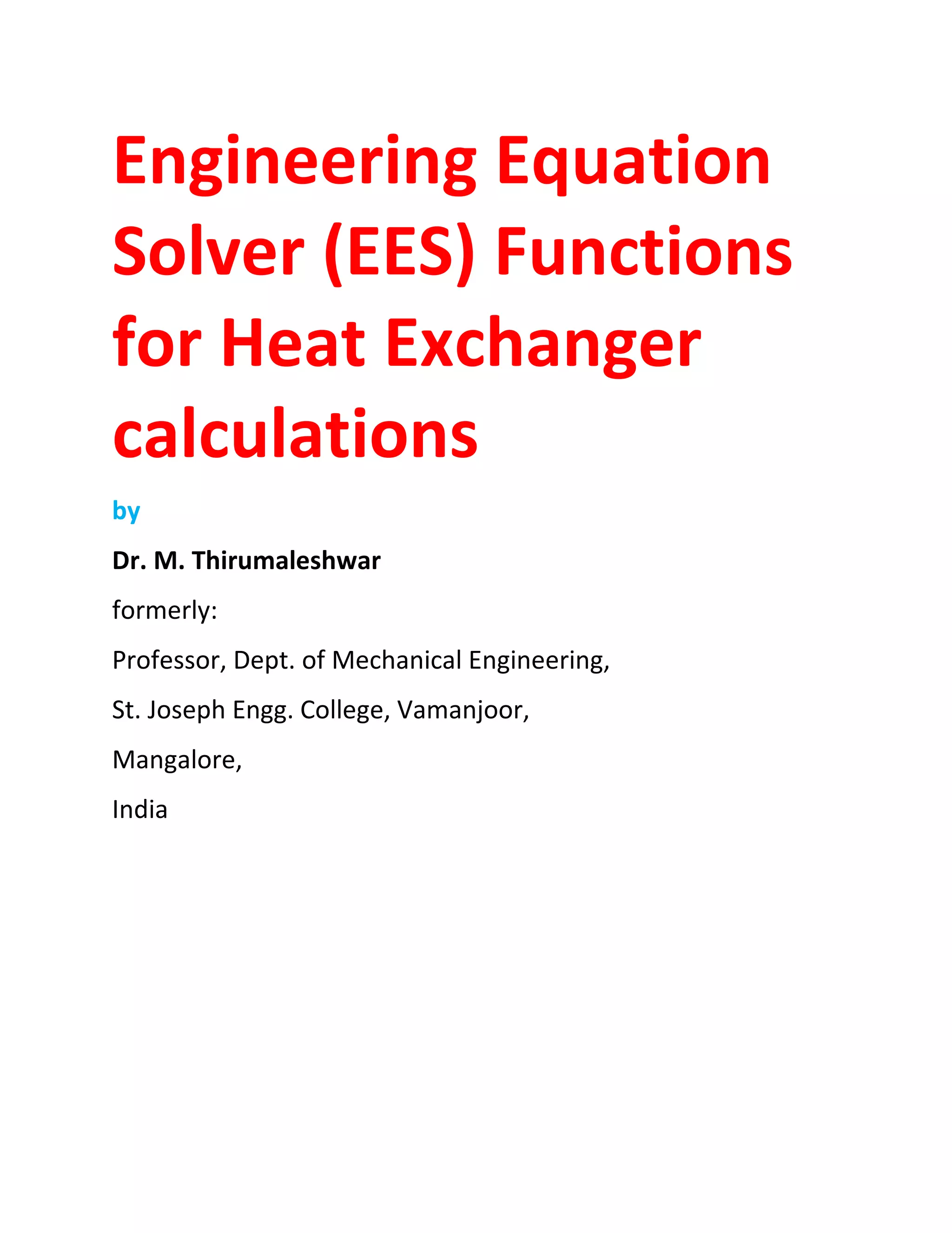
"Prob. B.1.1: A shell and tube counter-flow heat exchanger uses copper tubes (k = 380 W/(m.C)), 20 mm
ID and 23 mm OD. Inside and outside film coefficients are 5000 and 1500 W/(m2.C) respectively.
Fouling factors on the inside and outside may be taken as 0.0004 and 0.001 m2.C/W respectively.
Calculate the overall heat transfer coefficient based on: (i) outside surface, and (ii) inside surface."
"Data:"
D_i = 0.02 [m]
D_0 = 0.023 [m]
L = 1 [m]
k_wall = 380 [W/m_C]
h_i = 5000 [W/m^2-C] "...heat tr coeff on the inside"
h_0 = 1500 [W/m^2-C] "...heat tr coeff on the outside"
R_fi = 0.0004 [m^2-C/W] "...Fouling factor on the inside"

8. R_f0 = 0.001 [m^2-C/W] "...Fouling factor on the outside"
"Calculations:"
CALL Overall_U_cyl ( L, k_wall, D_i, D_0, h_i, h_0, R_fi, R_f0: R_cond, R_i, R_0, R_ci, R_c0, R_tot,U_i,
U_0)
"======================================================================="
* "
"
H6 0 =2A ( < - I& 5 J %
H6' 0 =&1 ) < - I& 5J %
% , $ *6 # H6' . &' ='' < - 5"
, $ ! "

9. D , $ "

10. $$ $ # "
# H6 # H6' &,
*6 # *6 ' K "
! *6 0 ' # *6 ' 0 ', # $ , "
"
H6 0 (&AA < - I& 5 , J %
H6' 0 (((' < - I& 5, J %

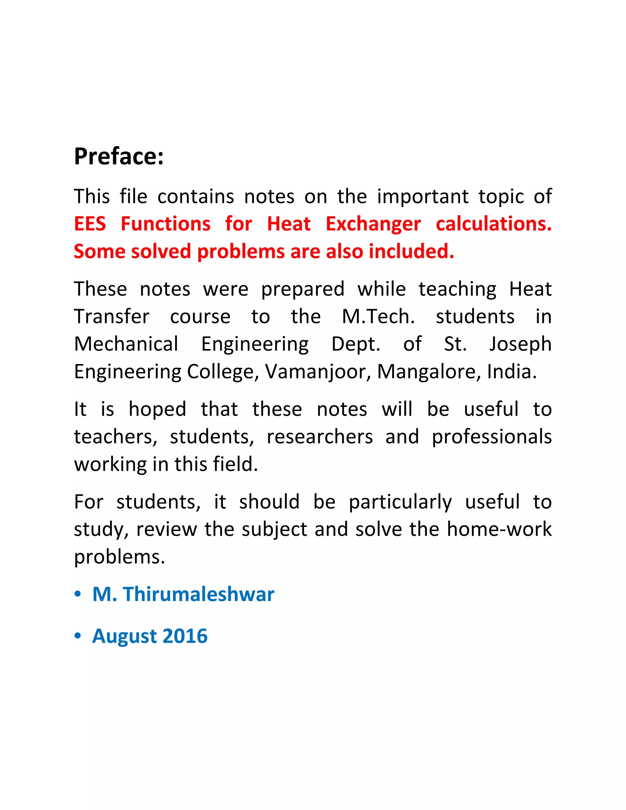
11. "Prob. B.1.2: Consider a type 302 SS tube (k = 15.10 W/(m.C)), 22 mm ID and 27 mm OD, inside
which water flows at a mean temp T_m = 75 C and velocity u_m = 0.5 m/s. Air at 15 C and at a velocity
of V_0 = 20 m/s flows across this tube. Fouling factors on the inside and outside may be taken as 0.0004
and 0.0002 m^2.C/W respectively. Determine the overall heat transfer coefficient based on the outside
surface, U_0 (b) Plot U_o as a function of cross flow velocity, V_0 in the range: 5 < V_o < 30 m/s."
"EES Solution:"
"Data:"
D_i = 0.022 [m]
D_0 = 0.027 [m]
L = 1 [m]
k_wall = 15.1 [W/m-C]
T_m_water = 75 [C]
U_m_water = 0.5 [m/s]
P_1 = 1.01325E05 [Pa]
T_m_air = 15 [C]
V_0_air = 20 [m/s]
"Properties of Water at T_m:"
rho_w=Density(Steam_IAPWS,T=T_m_water,P=P_1)
mu_w=Viscosity(Steam_IAPWS,T=T_m_water,P=P_1)
cp_w=SpecHeat(Steam_IAPWS,T=T_m_water,P=P_1)
k_w=Conductivity(Steam_IAPWS,T=T_m_water,P=P_1)
Pr_w=Prandtl(Steam_IAPWS,T=T_m_water,P=P_1)
"Calculations:"
"To determine inside heat transfer coeff. h_i:"
Re_water = D_i * U_m_water * rho_w / mu_w "...finds Reynolds No. for water"
"Re_water = 28388 > 4000; So, apply Dittus - Boelter eqn to find out Nusselts No.:"
Nusselts_w = 0.023 * Re_water^0.8 * Pr_w^0.4 "...gives Nusselts No."
Nusselts_w = h_i * D_i /k_w "....finds h_i, heat tr coeff on the inside "
"To determine outside heat transfer coeff. h_0:"
"It is cross flow of air across a cylinder. So, use the EES PROCEDURE written above to find out h_0,
using the Churchill - Bernstein eqn for cross flow of a fluid over a cylinder:"

12. Fluid$ = 'Air'
P_infinity = P_1
T_infinity = 15[C]
U_infinity = V_0_air
D = D_0
{T_s = 70 "[C] .... assumed, will be corrected later"}
CALL ForcedConv_AcrossCylinder (Fluid$,P_infinity, T_infinity, U_infinity, L, D, T_s: Re_D,
Nusselt_D_bar, h_0, Q)
R_fi = 0.0004 [m^2-C/W] "...Fouling factor on the inside"
R_f0 = 0.0002 [m^2-C/W] "...Fouling factor on the outside"
CALL Overall_U_cyl ( L, k_wall, D_i, D_0, h_i, h_0, R_fi, R_f0: R_cond, R_i, R_0, R_ci, R_c0, R_tot, U_i,
U_0)
{(T_s - T_m_air) / R_conv_out = (T_m_water - T_s) / (R_conv_in + R_c_in + R_cond_wall + R_c_out)
"....finds T_s, the surface temp of cylinder"}
(T_s - 15[C]) / R_0 = (T_m_water - T_s) / (R_i +R_ci + R_cond + R_c0) "Finds surface temp on the
fouling layer on the outer surface of the tube "
U_i * A_i = 1 / R_tot "...determine U _i"
U_0 * A_0 = 1 / R_tot "...determine U _0"
Results:

13. "
H6 0 ((& A < - I& 5 J %
H6' 0 @( 2 < - I& 5 J %
! H6' % # "
, $ ! "
D , $ "

14. 3 & ; # # , ; 5
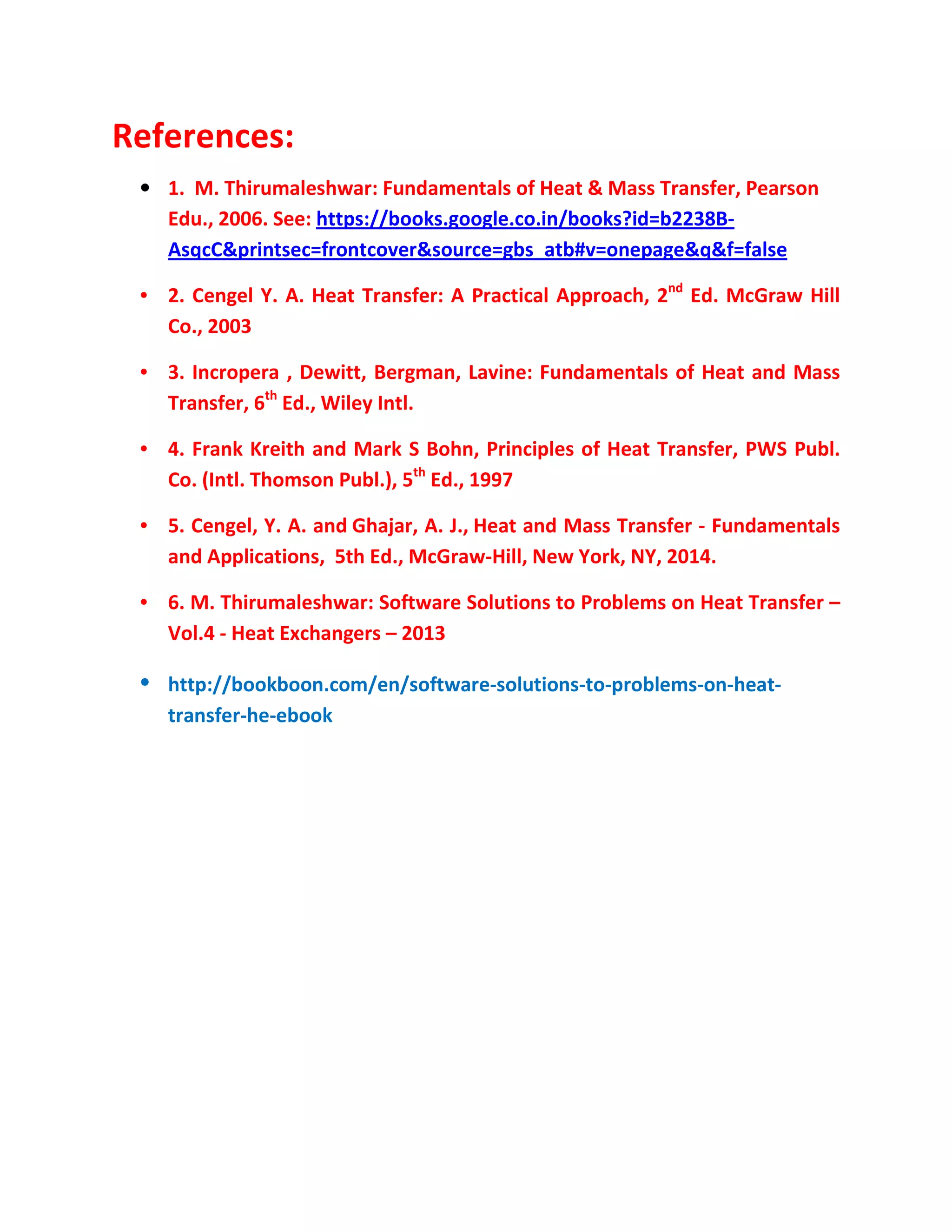
"Prob. B.2.1. A HX is required to cool 55000 kg/h of alcohol from 66 C to 40 C using 40000 kg/h of
water entering at 5 C. Calculate the following: (i) the exit temp of water (ii) surface area required for
parallel flow and counter-flow HXs. Take U = 580 W/m^2.K, cp for alcohol = 3760 J/kg.K, cp for water
= 4180 J/kg.K. [VTU -May - June- 2006]"
Fig. Prob.B.2.1(a).Counter-flow arrangement
Fig. Prob.B.2.1(b).Parallel flow arrangement
EES Solution:
"Data:"
m_h = 55000 [kg/h] * convert (kg/h, kg/s) "...hot fluid---alcohol"
m_c = 40000 [kg/h] * convert (kg/h, kg/s) "....cold fluid -- water"
T_h_i = 66 [C]
T_c_i = 5 [C]
T_h_o = 40 [C]
cp_h = 3760 [J/kg-C]

15. cp_c = 4180 [J/kg-C]
U= 580 [W/m^2-C]
"Calculations:"
"Exit temp of cold fluid:"
m_h * cp_h * (T_h_i - T_h_o) = m_c * cp_c * (T_c_o - T_c_i) " C...determines T_c_o"
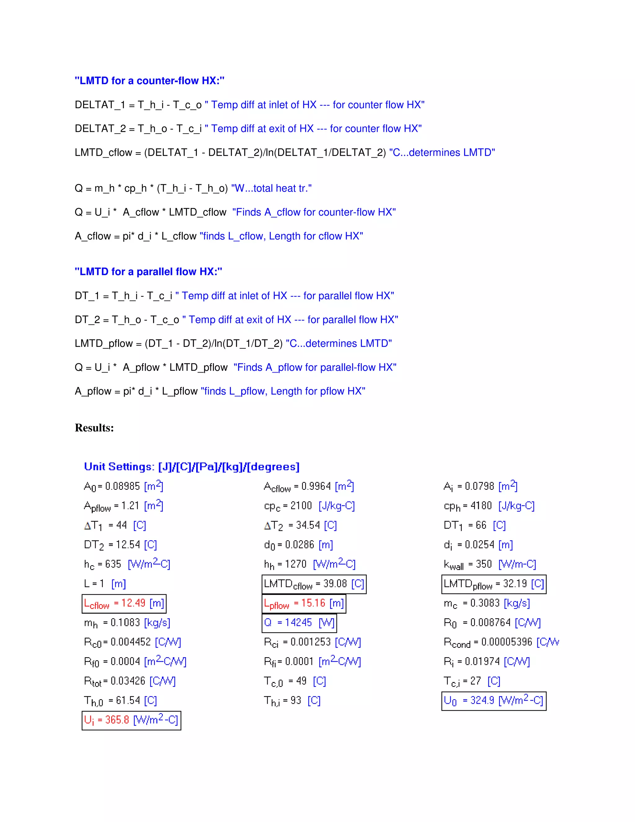
"LMTD for a counter-flow HX:"
DELTAT_1 = T_h_i - T_c_o " Temp diff at inlet of HX --- for counter flow HX"
DELTAT_2 = T_h_o - T_c_i " Temp diff at exit of HX --- for counter flow HX"
LMTD_cflow = (DELTAT_1 - DELTAT_2)/ln(DELTAT_1/DELTAT_2) "C...determines LMTD"
Q = m_h * cp_h * (T_h_i - T_h_o) "W...heat tr."
Q = U * A_cflow * LMTD_cflow "Finds A_cflow for counter-flow HX"
"LMTD for a parallel flow HX:"
DT_1 = T_h_i - T_c_i " Temp diff at inlet of HX --- for parallel flow HX"
DT_2 = T_h_o - T_c_o " Temp diff at exit of HX --- for parallel flow HX"
LMTD_pflow = (DT_1 - DT_2)/ln(DT_1/DT_2) "C...determines LMTD"
Q = U * A_pflow * LMTD_pflow "Finds A_pflow for parallel-flow HX"
Results:
Thus:
Exit temp of water = 37.16 C … Ans.
Area for parallel flow HX = 135.8 m^2 …. Ans.
Area for counter-flow HX = 80.92 m^2 …. Ans.
--------------------------------------------------------------------------------------------------------------

16. Prob. B.2.2. Sat. steam at 120 C is condensing on the outer surface of a single pass HX. The overall heat
transfer coeff is 1600 W/m^2.C. Determine the surface area of the HX required to heat 2000 kg/h of water
from 20 C to 90 C. Also determine the rate of condensation of steam (kg/h). Assume latent heat of steam
as 2195 kJ/kg. [VTU-Aug. 2001]
Fig. Prob.B.2.2.
EES Solution:
"Data:"
m_c = 2000 [kg/h] * convert (kg/h, kg/s) "....cold fluid -- water"
T_h = 120 [C]
T_c_i = 20 [C]
T_c_o = 90 [C]
cp_c = 4180 [J/kg-C]
U= 1600 [W/m^2-C]
"LMTD for a condenser:"
DELTAT_1 = T_h - T_c_i " Temp diff at inlet "
DELTAT_2 = T_h - T_c_o " Temp diff at exit "
LMTD = (DELTAT_1 - DELTAT_2)/ln(DELTAT_1/DELTAT_2) "C...determines LMTD"
Q = m_c * cp_c * (T_c_o - T_c_i) "W....finds heat tr, Q"
Q = U * A * LMTD "Finds Area, A for condenser"
h_fg = 2195000 [J/kg] "...latent heat for steam condensing"
m_h * h_fg = Q " kg/s...determines mass of steam condensed"
m_steam_perhour = m_h * convert (kg/s, kg/h)
Results:

17. Thus:
Area of HX = A = 1.747 m^2 …. Ans.
Rate of condensation of steam = 266.6 kg/h … Ans.
"Prob. B.2.3. A simple HX consisting of two concentric passages is used for heating 1110 kg/h of oil (cp
= 2.1 kJ/kg.K) from 27 C to 49 C. The oil flows through the inner pipe made of copper (OD = 2.86 cm,
ID = 2.54 cm, k = 350 W/m.K) and the surface heat transfer coeff on the oil side is 635 W/m^2.K. The oil
is heated by hot water supplied at a rate of 390 kg/h with an inlet temp of 93 C. The water side heat
transfer coeff. is 1270 W/m^2.K. The fouling factors on the oil and water sides are 0.0001 and 0.0004
m^2.K/W respectively. What is the length of HX required for (i) parallel flow, and
(ii) counter-flow ? [VTU-Jan-Feb.- 2006]"
Fig. Prob.B.2.3(a)..Counter-flow arrangement
Fig. Prob.B.2.3(b)..Parallel flow arrangement

18. EES Solution:
"Data:"
m_h = 390 [kg/h] * convert (kg/h, kg/s) "...hot fluid---water"
m_c = 1110 [kg/h] * convert (kg/h, kg/s) "....cold fluid -- oil - flows through inner pipe"
T_h_i = 93 [C]"...inlet temp of hoy fluid"
T_c_i = 27 [C]"...inlet temp of cold fluid"
T_c_0 = 49[C] "...outlet temp of cold fluid"
cp_h = 4180 [J/kg-C]
cp_c = 2100 [J/kg-C]
h_h = 1270[W/m^2-C]
h_c = 635[W/m^2-C]
d_i = 0.0254[m]
d_0 = 0.0286[m]
k_wall = 350 [W/m-C]
R_fi = 0.0001[m^2-C/W]
R_f0 = 0.0004[m^2-C/W]
L = 1[m]"...assumed"
A_i = pi * d_i * L "[m^2]....inside surface area"
A_0 = pi * d_0 * L "[m^2]....outside surface area"
"Calculations:"
"Overall heat tr coeff."
CALL Overall_U_cyl ( L, k_wall, d_i, d_0, h_c, h_h, R_fi, R_f0: R_cond, R_i, R_0, R_ci, R_c0, R_tot, U_i,
U_0) "..here, we get U_i and U_0 "
Running the above program, we get U_i:
i.e. U_i = 365.8 W/m^2.C .. Ans.
Continuing the program:
m_h * cp_h * (T_h_i - T_h_o) = m_c * cp_c * (T_c_o - T_c_i) " C...determines T_h_o"

19. "LMTD for a counter-flow HX:"
DELTAT_1 = T_h_i - T_c_o " Temp diff at inlet of HX --- for counter flow HX"
DELTAT_2 = T_h_o - T_c_i " Temp diff at exit of HX --- for counter flow HX"
LMTD_cflow = (DELTAT_1 - DELTAT_2)/ln(DELTAT_1/DELTAT_2) "C...determines LMTD"
Q = m_h * cp_h * (T_h_i - T_h_o) "W...total heat tr."
Q = U_i * A_cflow * LMTD_cflow "Finds A_cflow for counter-flow HX"
A_cflow = pi* d_i * L_cflow "finds L_cflow, Length for cflow HX"
"LMTD for a parallel flow HX:"
DT_1 = T_h_i - T_c_i " Temp diff at inlet of HX --- for parallel flow HX"
DT_2 = T_h_o - T_c_o " Temp diff at exit of HX --- for parallel flow HX"
LMTD_pflow = (DT_1 - DT_2)/ln(DT_1/DT_2) "C...determines LMTD"
Q = U_i * A_pflow * LMTD_pflow "Finds A_pflow for parallel-flow HX"
A_pflow = pi* d_i * L_pflow "finds L_pflow, Length for pflow HX"
Results:

20. Thus:
Length of HX for parallel flow HX = L_pflow = 15.16 m …. Ans.
Length of HX for counter-flow HX = L_cflow = 12.49 m … Ans.
---------------------------------------------------------------------------------------------------------
!*G 5 H* # ; +
"
Let us write EES PROCEDURE to find LMTD_CF and F for a Shell & Tube HX:
We recollect:
Equations:
If R is not equal to 1:
If R = 1:

21. In the above, N is the no. of simple shells or no. of shell passes.
-----------------------------------------------------------------------------------------------------
Following is the EES Procedure:
$UnitSystem SI Pa C J
PROCEDURE Shell_and_TubeHX_LMTD_F(Tshell_1,Tshell_2,Ttube_1,Ttube_2,N :
R,P,F,LMTD_CF,LMTD_corrected)
"Gives R, P, F, LMTD_CF and LMTD_corrected as output:"
"Input: Inlet and exit temps of Shell side and Tube side fluids, and N is the no. of simple shells or no. of
Shell passes"
DT1 := Tshell_1 - Ttube_2
DT2 := Tshell_2 - Ttube_1
LMTD_CF := ABS(DT1 - DT2) / ABS (ln (DT1/DT2))
P := (Ttube_2 - Ttube_1) / (Tshell_1 - Ttube_1)
R := (Tshell_1 - Tshell_2) / (Ttube_2 - Ttube_1)
IF (Tshell_1 = Tshell_2) OR (Ttube_1 = Ttube_2) THEN
F := 1
LMTD_corrected := F * LMTD_CF
RETURN
ENDIF
IF ( R = 1) THEN
X := P / (N - N * P + P)
F := (X * sqrt(2)) / ((1 - X) * ln( (2 * (1 - X) + x * sqrt(2)) / (2 * (1 - X) - x * sqrt(2))))
ENDIF
IF ( R <> 1) THEN
X :=(1 - ((R * P -1) / ( P - 1))^ (1/N)) / ( R - ((R * P -1)/(P - 1))^(1/N))
F := (sqrt(R^2 + 1) / ( R - 1)) * ln ((1 - X) / (1 - R * X)) / ln ((2/X - 1 - R + sqrt(R^2 + 1)) / (2/X - 1 - R -
sqrt(R^2 + 1)))
ENDIF
LMTD_corrected := F * LMTD_CF

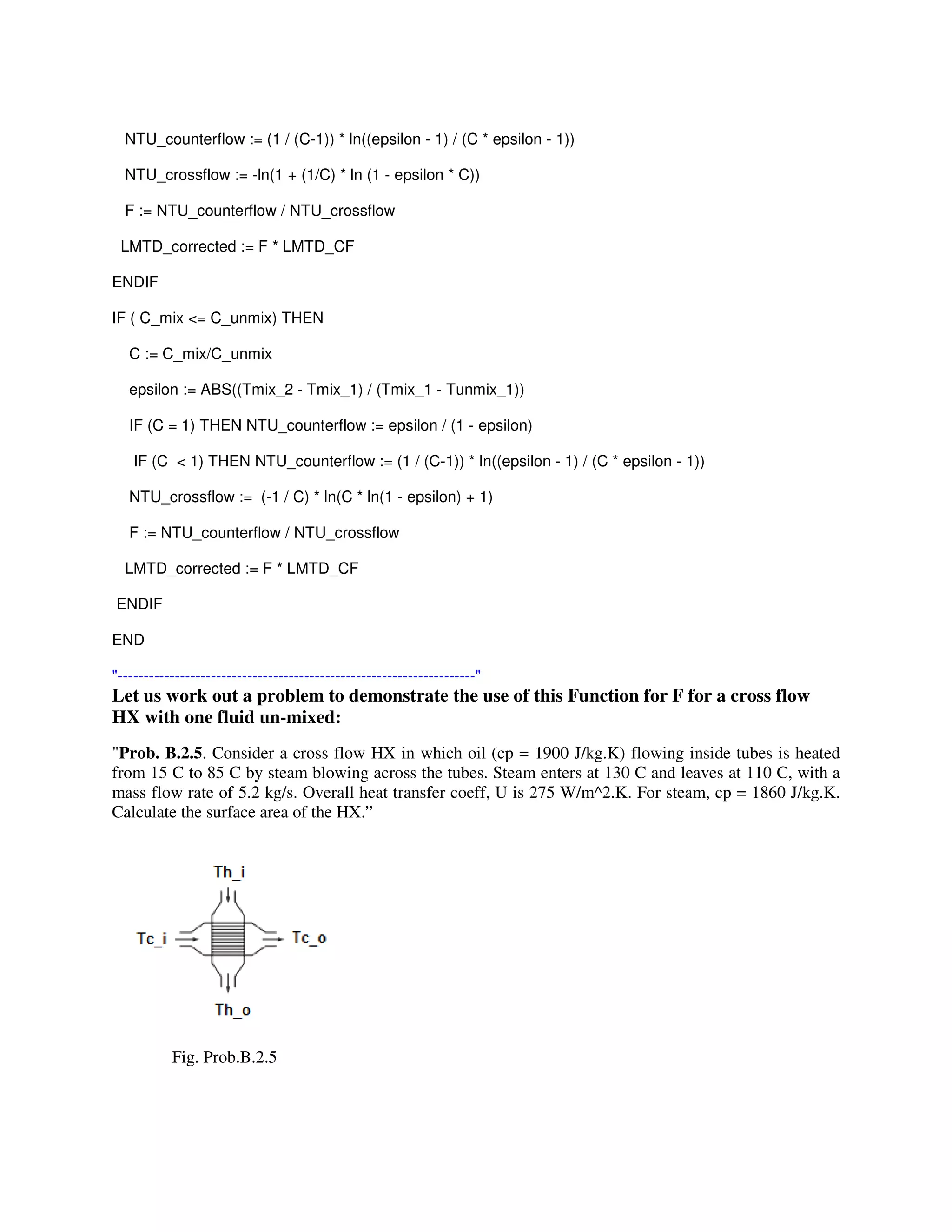
22. END
"---------------------------------------------------------------------"
Let us use this PROCEDURE to solve the following problem:
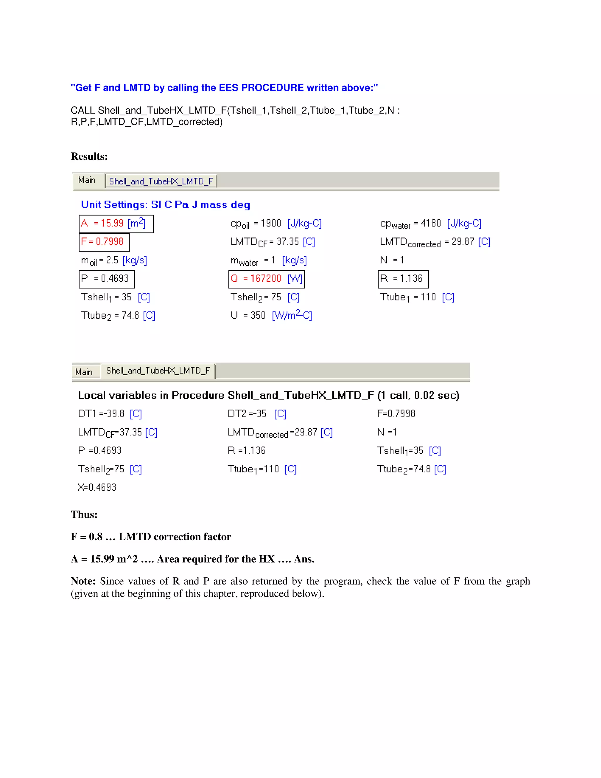
Prob. B.2.4. In a Shell & Tube HX, water, making one Shell pass, at a rate of 1 kg/s is heated from 35 to
75 C by an oil of sp. heat 1900 J/kg.C. Oil flows at a rate of 2.5 kg/s through the tubes making 2 passes
and enters the Shell at 110 C. If the overall heat transfer coeff. U is 350 W/m^2.C, calculate the area
required."
Fig. Prob.B.2.4. Temp profile for Counter-flow arrangement
EES Solution:
"Data:"
Tshell_1 = 35[C]"....inlet temp of water"
Tshell_2 = 75 [C]"....exit temp of water"
Ttube_1 =110 [C]"....inlet temp of oil"
m_water = 1 [kg/s]
cp_water = 4180 [J/kg-C]
m_oil = 2.5 [kg/s]
cp_oil = 1900 [J/kg-C]
U = 350 [W/m^2-C]
N = 1
"Calculation:"
"Total heat transferred, Q:"
Q = m_water * cp_water * (Tshell_2 - Tshell_1) "[W]"
Q = m_oil * cp_oil * (Ttube_1 - Ttube_2)"[C]...finds exit temp of oil, Ttube_2"
"Also:"
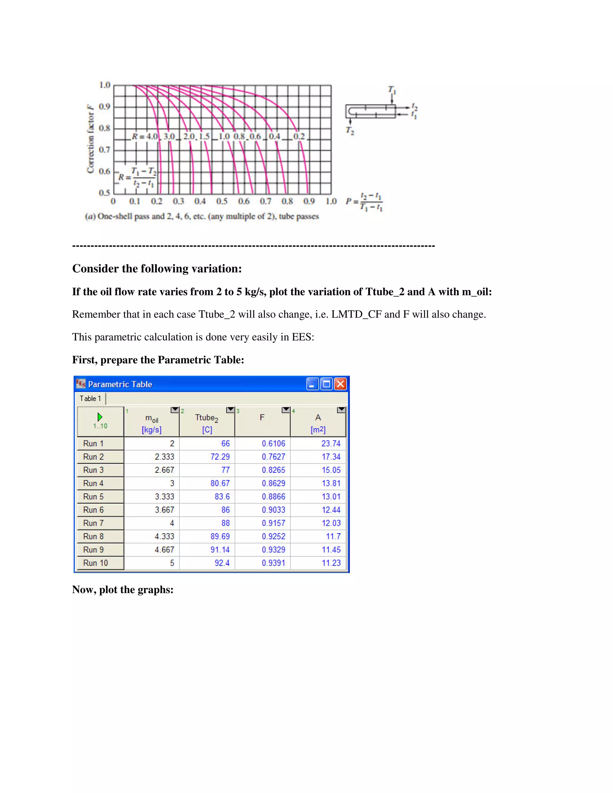
Q = U * A * F * LMTD_CF "...where F is the LMTD correction factor, and LMTD_CF is the LMTD for a true
counter-flow HX"

23. "Get F and LMTD by calling the EES PROCEDURE written above:"
CALL Shell_and_TubeHX_LMTD_F(Tshell_1,Tshell_2,Ttube_1,Ttube_2,N :
R,P,F,LMTD_CF,LMTD_corrected)
Results:
Thus:
F = 0.8 … LMTD correction factor
A = 15.99 m^2 …. Area required for the HX …. Ans.
Note: Since values of R and P are also returned by the program, check the value of F from the graph
(given at the beginning of this chapter, reproduced below).

24. ---------------------------------------------------------------------------------------------------
Consider the following variation:
If the oil flow rate varies from 2 to 5 kg/s, plot the variation of Ttube_2 and A with m_oil:
Remember that in each case Ttube_2 will also change, i.e. LMTD_CF and F will also change.
This parametric calculation is done very easily in EES:
First, prepare the Parametric Table:
Now, plot the graphs:

25. ========================================================

26. !*G 5 H* # ; L
# M #N, # M #N"
$UnitSystem SI Pa C J
PROCEDURE Crosssflow_OneMixed_LMTD_F(Tmix_1,Tmix_2,Tunmix_1,Tunmix_2,C_mix,C_unmix :
LMTD_CF,P,R,F,LMTD_corrected)
"Gives P, R, F, LMTD_CF and LMTD_corrected as output:
F is the LMTD correction factor. R and P are also output; so, F can be verified from the chart too."
"Input: Inlet and exit temps of mixed and unmixed fluids, andCmix and Cunmix are capacity rates of
respective fluids"
DT1 := Tmix_1 - Tunmix_2
DT2 := Tmix_2 - Tunmix_1
LMTD_CF := ABS(DT1 - DT2) / ABS (ln (DT1/DT2))
P := (Tunmix_2 - Tunmix_1) / (Tmix_1 - Tunmix_1)
R := (Tmix_1 - Tmix_2) / (Tunmix_2 - Tunmix_1)
IF (Tmix_1 = Tmix_2) OR (Tunmix_1 = Tunmix_2) THEN
F := 1
LMTD_corrected := F * LMTD_CF
RETURN
ENDIF
IF ( C_unmix < C_mix) THEN
C := C_unmix/C_mix
epsilon := ABS((Tunmix_2 - Tunmix_1) / (Tmix_1 - Tunmix_1))

27. NTU_counterflow := (1 / (C-1)) * ln((epsilon - 1) / (C * epsilon - 1))
NTU_crossflow := -ln(1 + (1/C) * ln (1 - epsilon * C))
F := NTU_counterflow / NTU_crossflow
LMTD_corrected := F * LMTD_CF
ENDIF
IF ( C_mix <= C_unmix) THEN
C := C_mix/C_unmix
epsilon := ABS((Tmix_2 - Tmix_1) / (Tmix_1 - Tunmix_1))
IF (C = 1) THEN NTU_counterflow := epsilon / (1 - epsilon)
IF (C < 1) THEN NTU_counterflow := (1 / (C-1)) * ln((epsilon - 1) / (C * epsilon - 1))
NTU_crossflow := (-1 / C) * ln(C * ln(1 - epsilon) + 1)
F := NTU_counterflow / NTU_crossflow
LMTD_corrected := F * LMTD_CF
ENDIF
END
"---------------------------------------------------------------------"
Let us work out a problem to demonstrate the use of this Function for F for a cross flow
HX with one fluid un-mixed:
"Prob. B.2.5. Consider a cross flow HX in which oil (cp = 1900 J/kg.K) flowing inside tubes is heated
from 15 C to 85 C by steam blowing across the tubes. Steam enters at 130 C and leaves at 110 C, with a
mass flow rate of 5.2 kg/s. Overall heat transfer coeff, U is 275 W/m^2.K. For steam, cp = 1860 J/kg.K.
Calculate the surface area of the HX.”
Fig. Prob.B.2.5

28. EES Solution:
"Data:"
Tmix_1 = 130 [C]
Tmix_2 = 110 [C]
Tunmix_1 = 15 [C]
Tunmix_2 = 85 [C]
cp_oil = 1900 [J/kg-C]
cp_steam = 1860 [J/kg-C]
m_steam = 5.2 [kg/s]
U = 275 [W/m^2 - C]
"Calculations:"
C_mix = m_steam * cp_steam "W/C... capacity rate of mixed fluid, i.e. steam"
Q = C_mix * (Tmix_1 - Tmix_2) "W"
C_unmix = Q / (Tunmix_2 - Tunmix_1) "W/C ...capacity rate of un-mixed fluid, i.e. oil"
"Using the EES Procedure written earlier:"
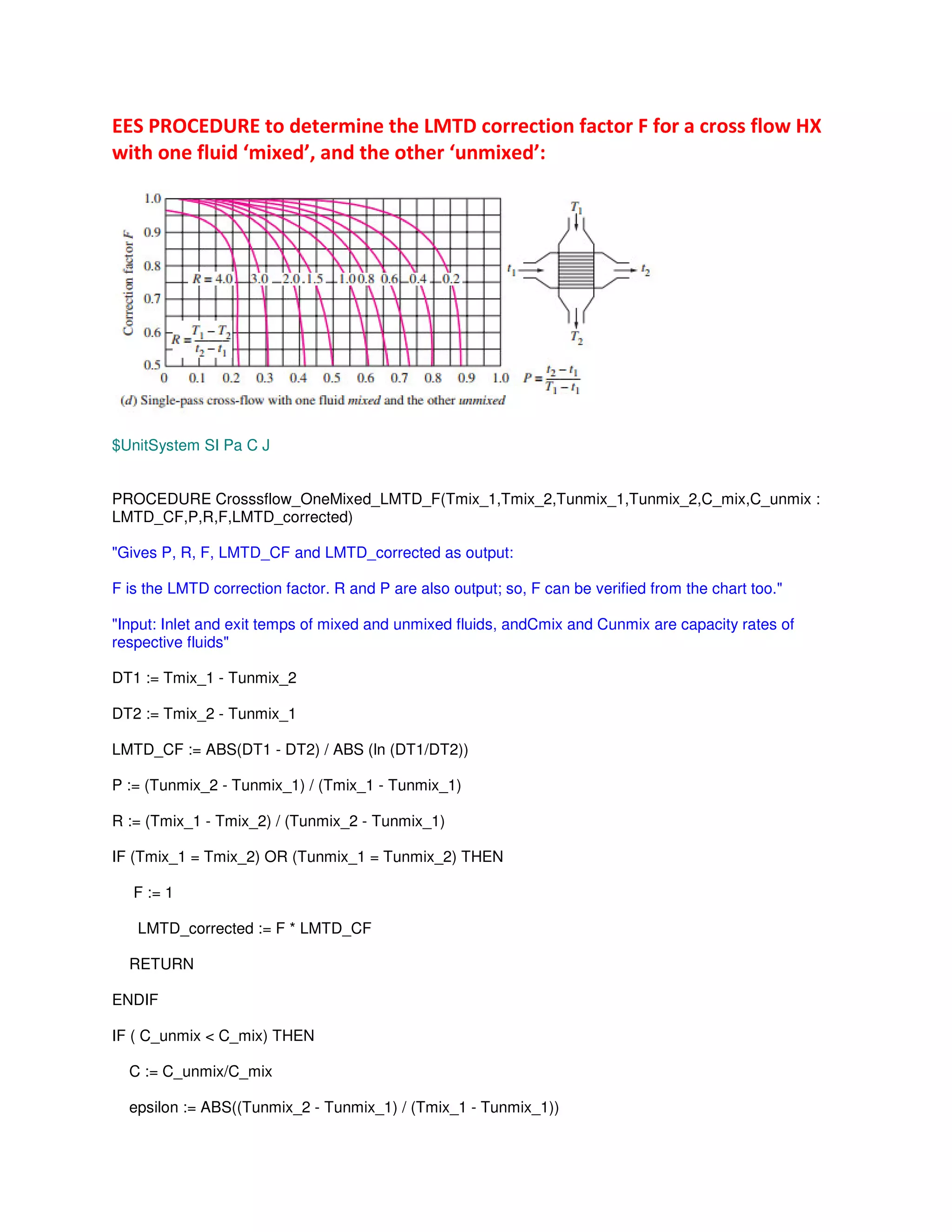
CALL Crosssflow_OneMixed_LMTD_F(Tmix_1,Tmix_2,Tunmix_1,Tunmix_2,C_mix,C_unmix :
LMTD_CF,P,R,F,LMTD_corrected)
Results:
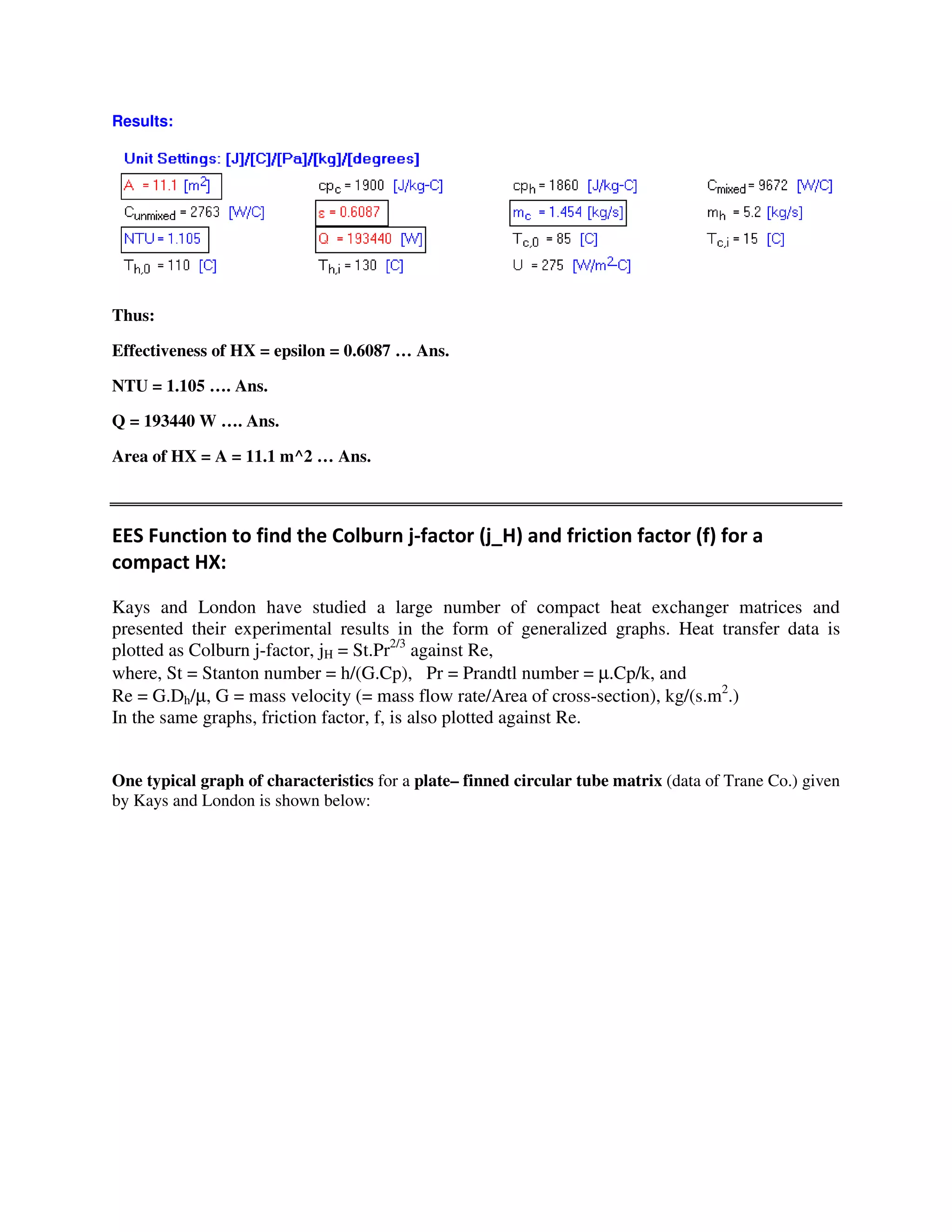
Thus:
LMTD correction factor, F = 0.9469
Area of HX, A = 11.1 m^2 …. Ans.
Note: Verify value of F from the graph given above.
=====================================================================

29. !*G 5 H* # ; L
# M #N"
We follow the following procedure:
We digitize each of the above graphs, i.e. for R = 4, 3, 2…0.2. And then, we curve fit each graph with
CurveExpert software and find the equation for each graph. Then, we write the EES Procedure to get F
for given P and R:
As an example, we show the curve fit eqn for R = 4:

31. Now, write the EES Function:
$UnitSystem SI Pa C J
PROCEDURE Crosssflow_BothUnmixed_LMTD_F(T_1,T_2,tt_1,tt_2,C_T,C_tt :
LMTD_CF,P,R,F,LMTD_corrected)
"Gives P, R, F, LMTD_CF and LMTD_corrected as output:
F is the LMTD correction factor. R and P are also output; so, F can be verified from the chart too."
"Input: Inlet and exit temps of fluid 1 (T) and fluid 2 (tt), and C_T and C_tt are capacity rates of respective
fluids"
P := (tt_2 - tt_1) / (T_1 - tt_1)
R := (T_1 - T_2) / (tt_2 - tt_1)
IF (R > 4) OR (R < 0.2) THEN
CALL ERROR ('R should be between 4 and 0.2. Here R is XXXF4', R)
ENDIF
DT1 := T_1 - tt_2
DT2 := T_2 - tt_1
LMTD_CF := ABS(DT1 - DT2) / ABS (ln (DT1/DT2))
IF (T_1 = T_2) OR (tt_1 = tt_2) THEN
F := 1
LMTD_corrected := F * LMTD_CF
RETURN
ENDIF
"For R = 4:"
a40 := 0.9672809; b40 := -4.0433204; c40 := -4.0064623; d40 := -0.3019396
F40 := (a40 + b40 * P)/(1+c40 * P + d40 * P^2)
"For R = 3:"
a30 :=1.0027344; b30 :=-2.9499251; c30 :=-2.8176633; d30 :=-0.059473011
F30 := (a30 + b30 * P)/(1+c30 * P + d30 * P^2)
"For R = 2:"
a20 :=1.0528796; b20:=-2.0982225; c20 :=-1.588803; d20 :=-0.66832947

32. F20 := (a20 + b20 * P)/(1+c20 * P + d20 * P^2)
"For R = 1.5:"
a15 :=1.013584; b15 :=-1.4982864; c15 :=-1.3928085; d15 :=0.1022294
F15 := (a15 + b15 * P)/(1+c15 * P + d15 * P^2)
"For R = 1:"
a10 :=1.0292657; b10 :=-0.23963952; c10 :=0.16670566; d10 :=0.31157928; e10 :=-1.4227221
F10 := (a10 + b10 * P + c10 * P^2 + d10 * P^3 + e10 * P^4)
"For R = 0.8:"
a08 :=1.007952; b08 :=-0.99036246; c08 :=-0.96731788; d08 :=0.14733358
F08 := (a08 + b08 * P)/(1+c08 * P + d08 * P^2)
"For R = 0.6:"
a06 :=1.0510175; b06 :=-1.0614768; c06 :=-0.84847439; d06 :=-0.099409186
F06 := (a06 + b06 * P)/(1+c06 * P + d06 * P^2)
"For R = 0.4:"
a04 :=1.0338023; b04 :=-1.0158388; c04 :=-0.87973396; d04 :=-0.061943671
F04 := (a04 + b04 * P)/(1+c04 * P + d04 * P^2)
"For R = 0.2:"
a02 :=1.016908; b02 :=-0.99564685; c02 :=-0.91765904; d02 :=-0.043092966
F02 := (a02 + b02 * P)/(1+c02 * P + d02 * P^2)
IF ((R >= 0.2) AND (R < 0.4)) THEN
F := F02 + (R - 0.2) * (F04 - F02) / (0.4 - 0.2)
ENDIF
IF ((R >= 0.4) AND (R < 0.6)) THEN
F := F04 + (R - 0.4) * (F06 - F04) / (0.6 - 0.4)
ENDIF
IF ((R >= 0.6) AND (R < 0.8)) THEN
F := F06 + (R - 0.6) * (F08 - F06) / (0.8 - 0.6)
ENDIF

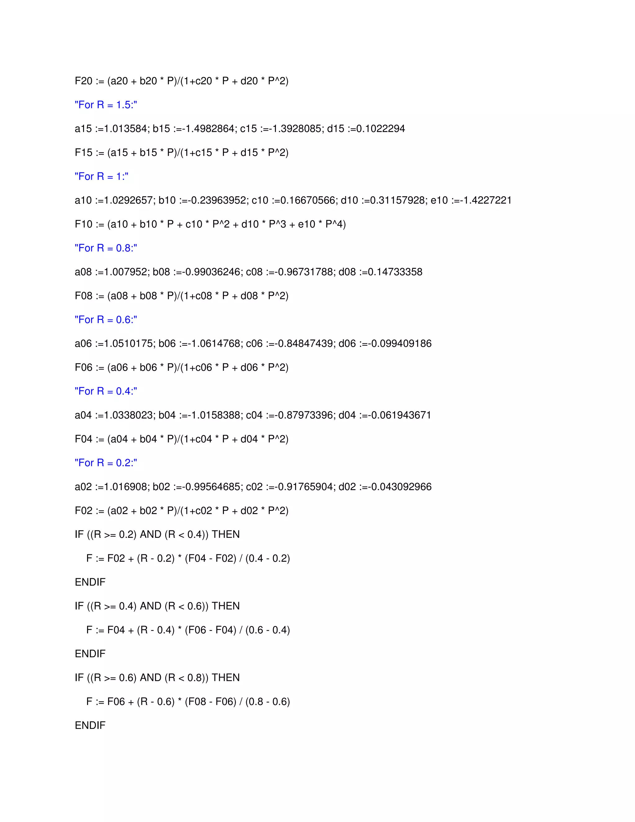
33. IF ((R >= 0.8) AND (R < 1)) THEN
F := F08 + (R - 0.8) * (F10 - F08) / (1 - 0.8)
ENDIF
IF ((R >= 1) AND (R < 1.5)) THEN
F := F10 + (R - 1) * (F15 - F10) / (1.5 - 1)
ENDIF
IF ((R >= 1.5) AND (R < 2)) THEN
F := F15 + (R - 1.5) * (F20 - F15) / (2 - 1.5)
ENDIF
IF ((R >= 2) AND (R < 3)) THEN
F := F20 + (R - 2) * (F30 - F20) / (3 - 2)
ENDIF
IF ((R >= 3) AND (R <= 4)) THEN
F := F30 + (R - 3) * (F40 - F30) / (4 - 3)
ENDIF
LMTD_corrected := F * LMTD_CF
END
"============================================================="
"Prob. B.2.6. A cross-flow HX in which both fluids are un-mixed is used to heat water with engine oil.
Water enter at 30 C and leaves at 85 C at a rate of 1.5 kg/s, while the engine oil with cp = 2.3 kJ/kg.C
enters at 120 C with a mass flow rate of 3.5 kg/s. The heat transfer surface area is 30 m^2. Calculate the
overall heat transfer coefficient by using the LMTD method. [VTU -June - July 2009]"
Fig. Prob.B.2.6.
Now, we shall solve this problem using the EES Function written above:

34. EES Solution:
"Data:"
m_h = 3.5 [kg/s] "...hot fluid---oil"
m_c = 1.5 [kg/s] "....cold fluid -- water"
T_h_i = 120 [C]
T_c_i = 30 [C]
T_c_o = 85 [C]
cp_h = 2300 [J/kg-C]
cp_c = 4180 [J/kg-C]
A = 30 [m^2]
m_h * cp_h * (T_h_i - T_h_o) = m_c * cp_c * (T_c_o - T_c_i) " C...determines T_h_o"
C_h = m_h * cp_h " W/C ... capacity ratre of hot fluid"
C_c = m_c * cp_c " W/C ... capacity ratre of cold fluid"
"To find LMTD Correction factor F for a cross-flow HX....
Either from the graph for a single pass HX with both fluids unmixed:, OR:
Use the EES Function written above"
CALL Crosssflow_BothUnmixed_LMTD_F(T_h_i,T_h_0,T_c_i,T_c_0,C_h,C_c :
LMTD_CF,P,R,F,LMTD_corrected)
Q = m_h * cp_h * (T_h_i - T_h_0) "W...heat tr."
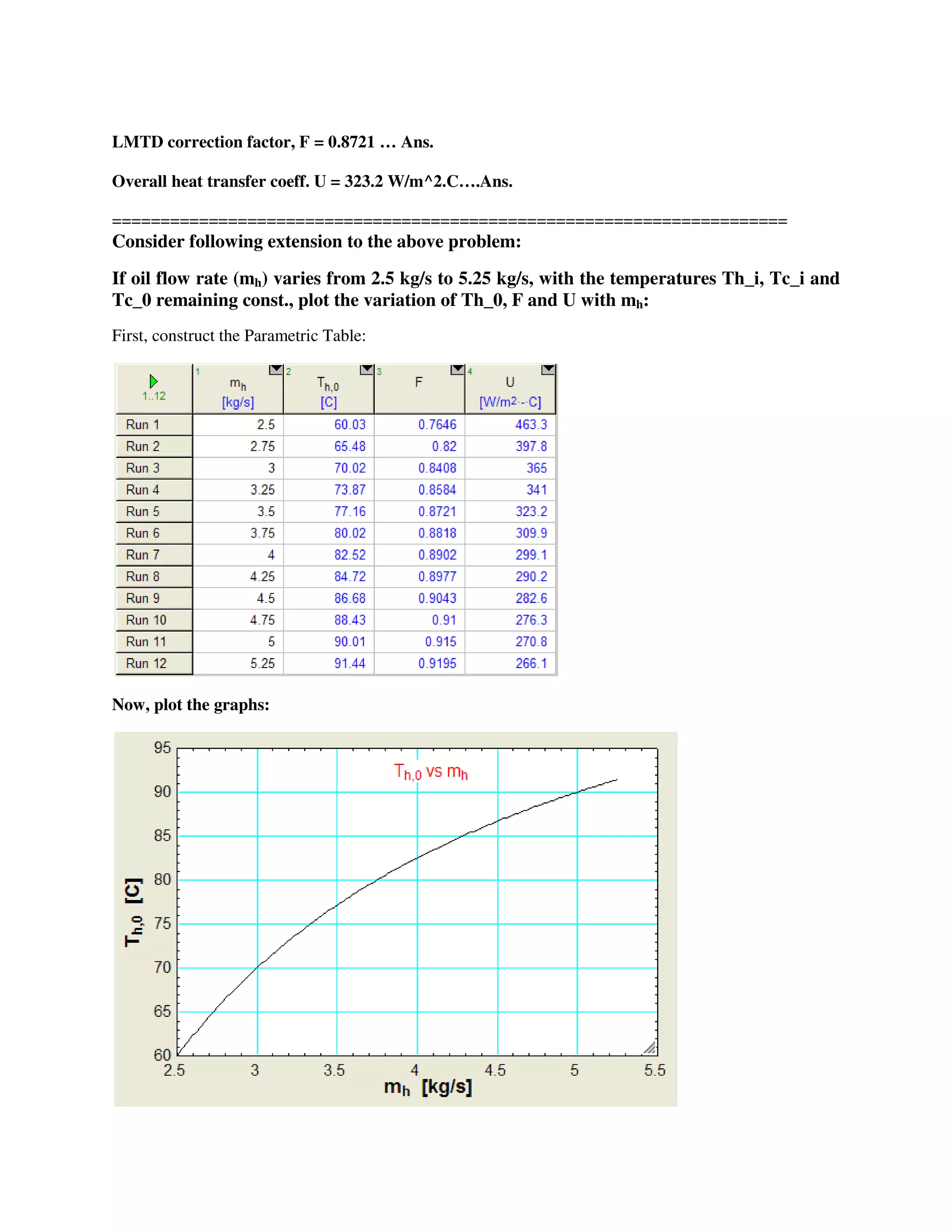
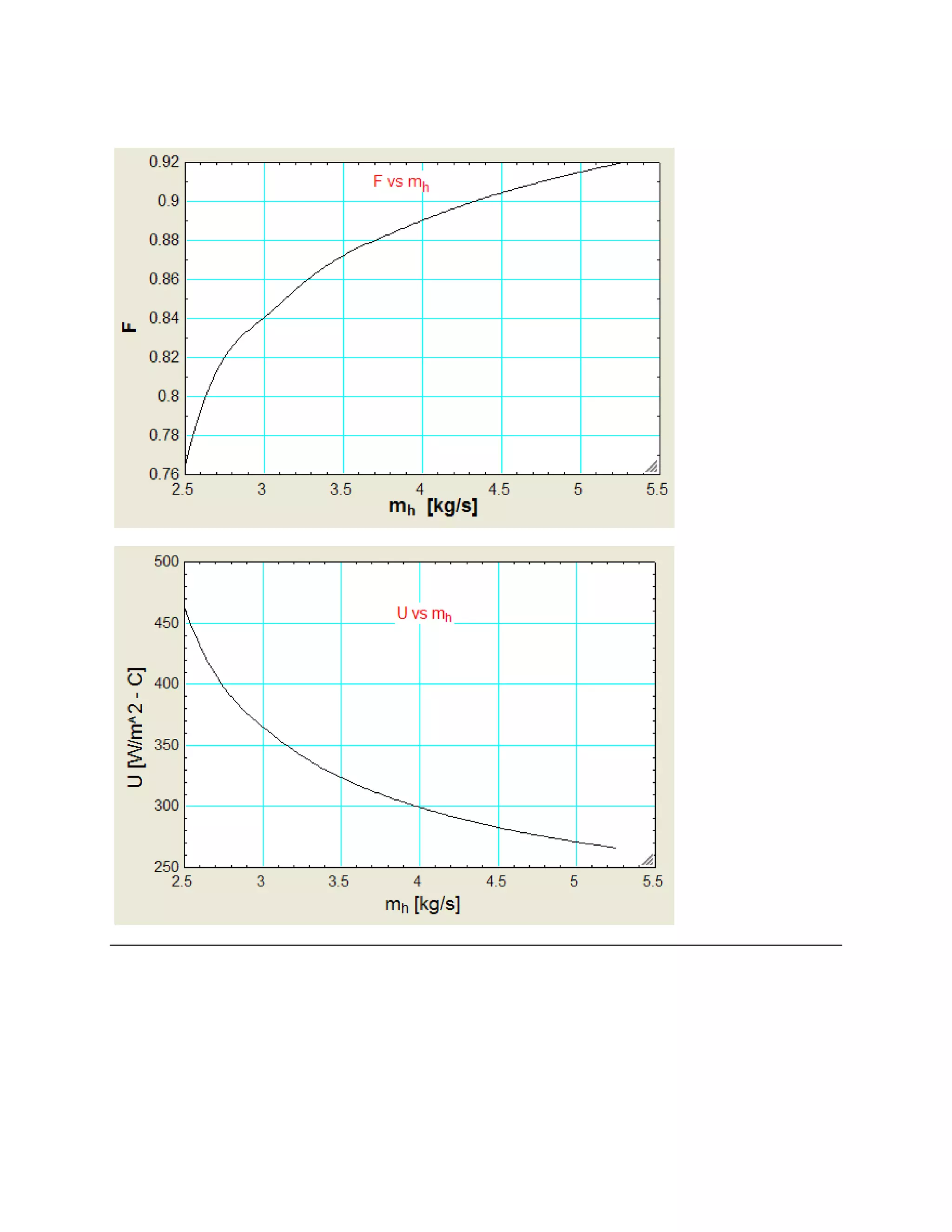
Q = U * A * LMTD_corrected "... Finds U"
"=============================================="
{Note: F = 0.87 approx. " From graph given above, for values of R and P given below:"}
Results:
Thus:

35. LMTD correction factor, F = 0.8721 … Ans.
Overall heat transfer coeff. U = 323.2 W/m^2.C….Ans.
======================================================================
Consider following extension to the above problem:
If oil flow rate (mh) varies from 2.5 kg/s to 5.25 kg/s, with the temperatures Th_i, Tc_i and
Tc_0 remaining const., plot the variation of Th_0, F and U with mh:
First, construct the Parametric Table:
Now, plot the graphs:

37. 3 1 % MD H D H E
O N #"
# 5 L"
"Function to determine Effectiveness of Counterflow HX:"
FUNCTION Epsilon_CountreflowHX(NTU,C_r)
"Finds the effectiveness of Counterflow HX:
Input: NTU, Capacity ratio, C _r( = C_min/C_max)
Output: Effectiveness"
IF (C_r = 0) THEN
Epsilon_CountreflowHX =1 - exp(-NTU)
RETURN
ENDIF
IF (C_r = 1) THEN
Epsilon_CountreflowHX = NTU / (1 + NTU)
RETURN
ENDIF
IF ((C_r > 0) OR (C_r <1)) THEN
Epsilon_CountreflowHX = (1 - exp ( - NTU * (1 - C_r)))/(1 - C_r * exp( - NTU * (1 - C_r))) "Effectiveness
of Counterflow HX."
ENDIF
END
"======================================================"
# ! L"
"Function to determine Effectiveness of Parallel flow HX:"
FUNCTION Epsilon_ParallelflowHX(NTU,C_r)
"Finds the effectiveness of Parallelflow HX:
Input: NTU, Capacity ratio, C _r( = C_min/C_max)

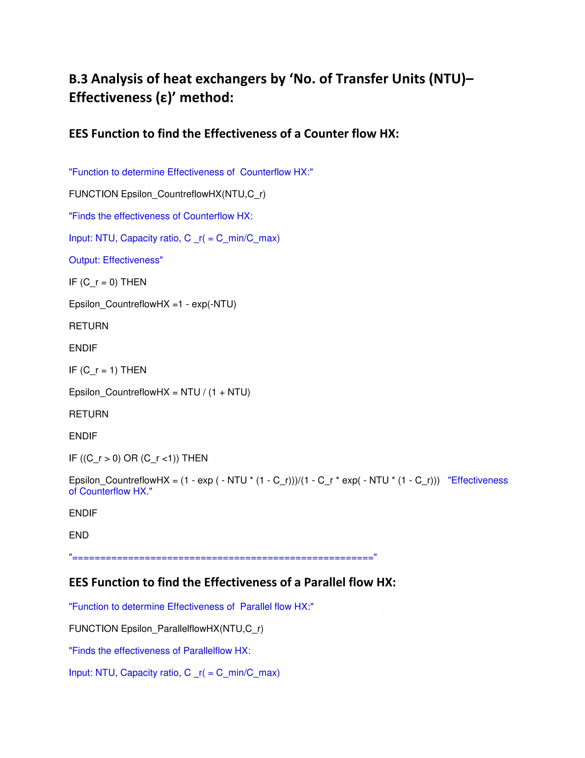
38. Output: Effectiveness"
IF (C_r = 0) THEN
Epsilon_ParallelflowHX =1 - exp(-NTU)
RETURN
ENDIF
IF ((C_r > 0) OR (C_r <=1)) THEN
Epsilon_ParallelflowHX = (1 - exp ( - NTU * (1 + C_r)))/(1 + C_r) "Effectiveness of Parallelflow HX."
ENDIF
END
"======================================================"
"Prob. B.3.1. A water to water HX of a counter-flow arrangement has a heating surface area of 2 m^2.
Mass flow rates of hot and cold fluids are 2000 kg/h and 1500 kg/h respectively. Temperatures of hot and
cold fluids at inlet are 85 C and 25 C respectively. Determine the amount of heat transferred from hot to
cold water and their temps at the exit if the overall heat transfer coeff. U = 1400 W/m^2.K. [VTU -May -
June 2010]:
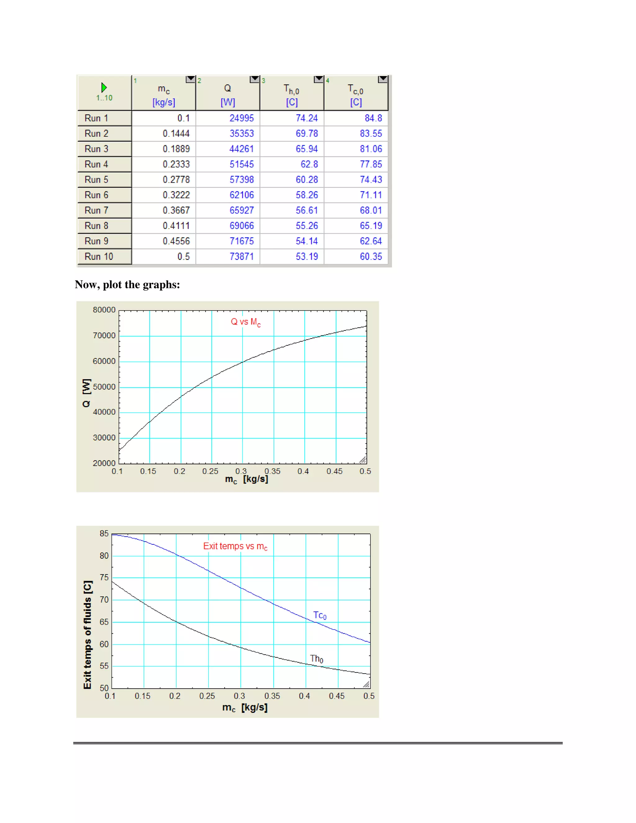
(b) Plot the variation of Q, Th_o and Tc_o as the mass flow rate of cold fluid, m_c varies from 0.1 to 0.5
kg/s. Assume other conditions to remain the same.”
Fig. Prob.B.3.1. Counter-flow arrangement
EES Solution:
"Data:"
m_h = 2000 [kg/h]* convert(kg/h, kg/s)
m_c = 1500 [kg/h] * convert(kg/h, kg/s)
T_h_i = 85 [C]

39. T_c_i = 25 [C]
cp_h = 4180 [J/kg-C]
cp_c = 4180 [J/kg-C]
U = 1400 [W/m^2-C]
A = 2 [m^2]
"Calculations:"
C_h = m_h * cp_h "W/C...=2322"
C_c = m_c * cp_c "W/C... = 1742 "
C_min = C_c
C_max = C_h
C_r = C_min/C_max
NTU = U * A/C_min "...calculates NTU"
"For counterflow HX: Use the EES Function for Effectiveness of Counterflow HX, written above"
epsilon = Epsilon_CountreflowHX(NTU,C_r) "Effectiveness of Counterflow HX."
"Also:"
epsilon = (T_c_0 - T_c_i) / (T_h_i - T_c_i) "...by definition, taking the min fluid... calculates Tc_0"
Q = m_h * cp_h * (T_h_i - T_h_0) "W...heat tr... calculates Th_0"
Q= m_c * cp_c * (T_c_0 - T_c_i) "W... calculates Q"
"============================================================="
Results:
Thus:
Q = 69418 W, Th_0 = 55.11 C, Tc_0 = 64.86 C .. Ans.
-----------------------------------------------------------------------------------------------------
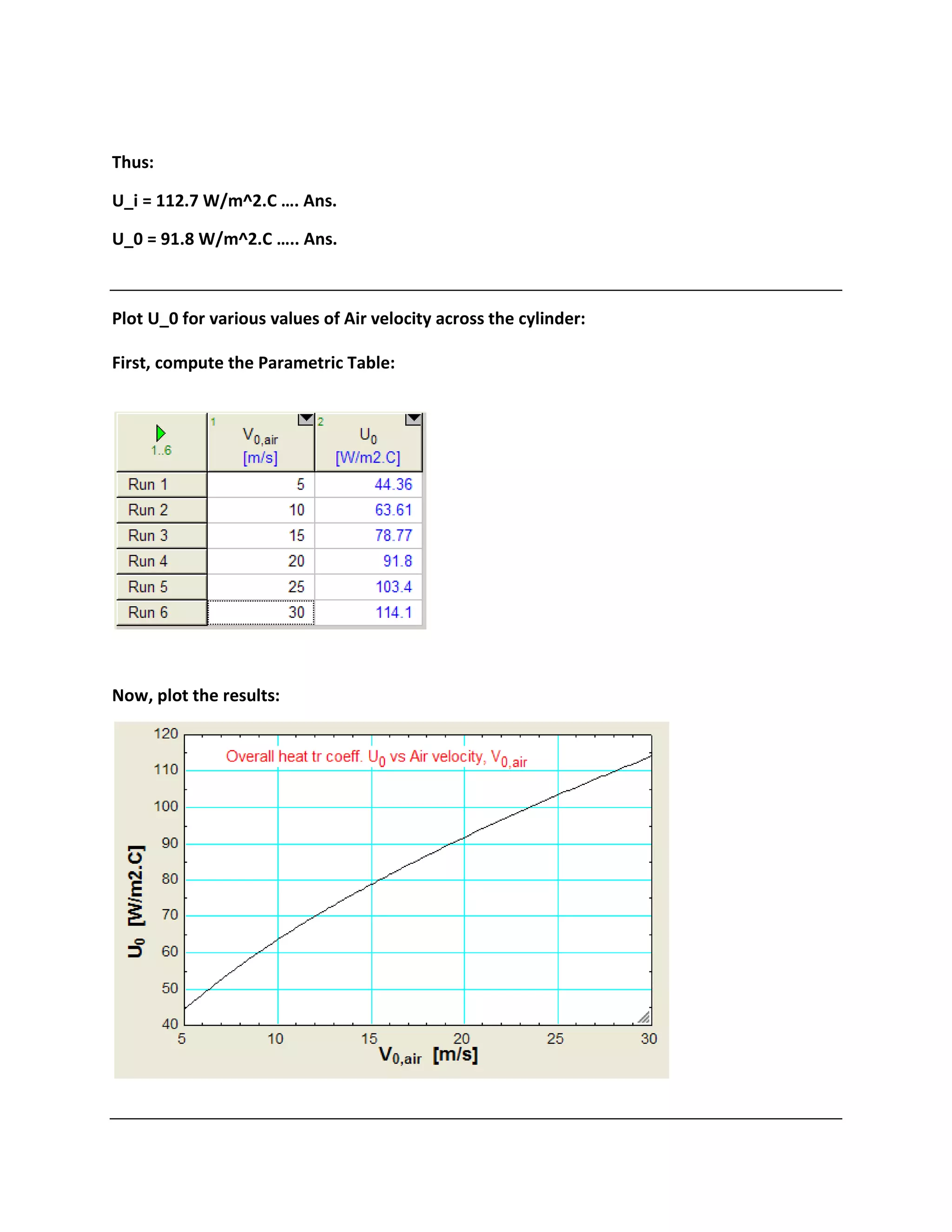
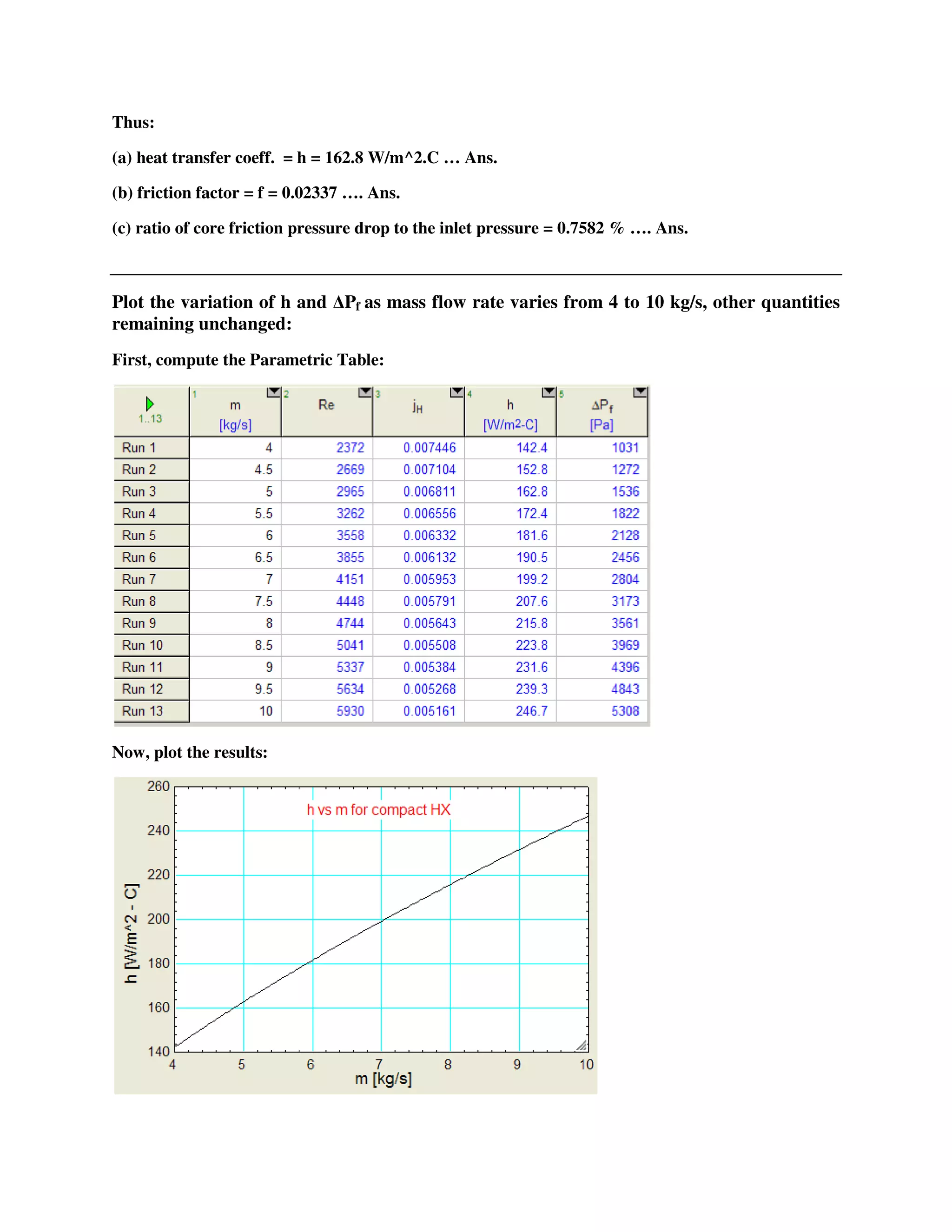
Plot the variation of Q, Th_o and Tc_o as the mass flow rate of cold fluid, m_c varies from
0.1 to 0.5 kg/s. Assume other conditions to remain the same:
First, compute the Parametric Table:

40. Now, plot the graphs:

41. “Prob. B.3.2. (M.U. 1995): Consider a heat exchanger for cooling oil which enters at 180 C, and cooling
water enters at 25 C. Mass flow rates of oil and water are: 2.5 and 1.2 kg/s, respectively. Area for heat
transfer = 16 m2. Sp. heat data for oil and water and overall U are given: Cpoil = 1900 J/kg.K; Cpwater =
4184 J/kg.K; U = 285 W/m2.K. Calculate outlet temperatures of oil and water for Parallel and counter-
flow HX.”
"
"Data:"
m_h = 2.5 [kg/s]
m_c = 1.2 [kg/s]
T_h_i = 180 [C]
T_c_i = 25 [C]
cp_h = 1900 [J/kg-C]
cp_c = 4184 [J/kg-C]
U = 285 [W/m^2-C]
A = 16 [m^2]
"Calculations:"
C_h = m_h * cp_h "W/C...=4750"
C_c = m_c * cp_c "W/C... = 5021 "
C_min = C_h
C_max = C_c
C_r = C_min/C_max
NTU = U * A/C_min "...calculates NTU"
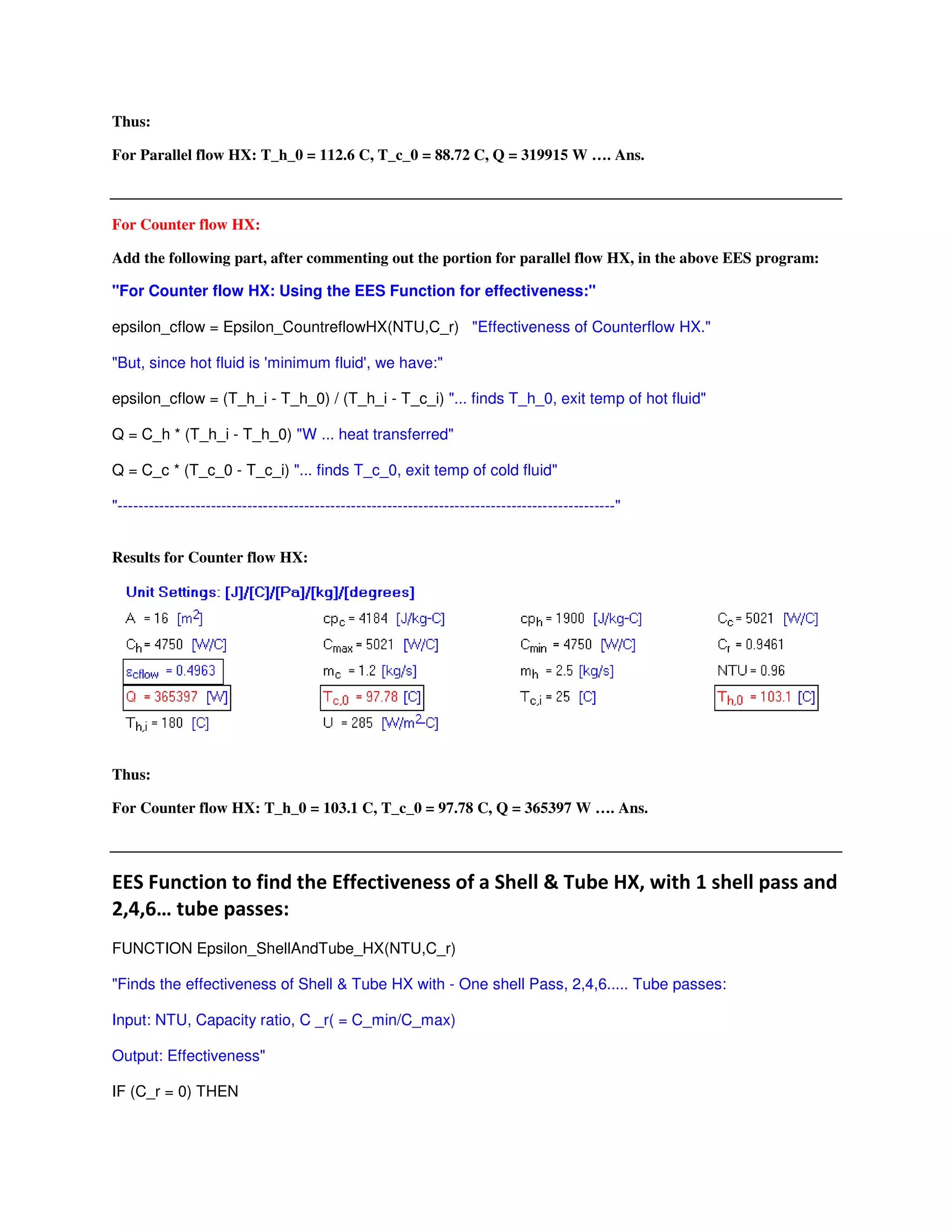
"For Parallel flow HX: Using the EES Function for effectiveness:"
epsilon_pflow = Epsilon_ParallelflowHX(NTU,C_r) "...finds effectiveness of parallel flow HX"
"But, since hot fluid is 'minimum fluid', we have:"
epsilon_pflow = (T_h_i - T_h_0) / (T_h_i - T_c_i) "... finds T_h_0, exit temp of hot fluid"
Q = C_h * (T_h_i - T_h_0) "W ... heat transferred"
Q = C_c * (T_c_0 - T_c_i) "... finds T_c_0, exit temp of cold fluid"
Results for Parallel flow HX:

42. Thus:
For Parallel flow HX: T_h_0 = 112.6 C, T_c_0 = 88.72 C, Q = 319915 W …. Ans.
For Counter flow HX:
Add the following part, after commenting out the portion for parallel flow HX, in the above EES program:
"For Counter flow HX: Using the EES Function for effectiveness:"
epsilon_cflow = Epsilon_CountreflowHX(NTU,C_r) "Effectiveness of Counterflow HX."
"But, since hot fluid is 'minimum fluid', we have:"
epsilon_cflow = (T_h_i - T_h_0) / (T_h_i - T_c_i) "... finds T_h_0, exit temp of hot fluid"
Q = C_h * (T_h_i - T_h_0) "W ... heat transferred"
Q = C_c * (T_c_0 - T_c_i) "... finds T_c_0, exit temp of cold fluid"
"------------------------------------------------------------------------------------------------"
Results for Counter flow HX:
Thus:
For Counter flow HX: T_h_0 = 103.1 C, T_c_0 = 97.78 C, Q = 365397 W …. Ans.
# + L, ( $ #
&,=,)J $ "
FUNCTION Epsilon_ShellAndTube_HX(NTU,C_r)
"Finds the effectiveness of Shell & Tube HX with - One shell Pass, 2,4,6..... Tube passes:
Input: NTU, Capacity ratio, C _r( = C_min/C_max)
Output: Effectiveness"
IF (C_r = 0) THEN

43. Epsilon_ShellAndTube_HX :=1 - exp(-NTU)
RETURN
ENDIF
IF ((C_r > 0) OR (C_r <=1)) THEN
AA := 1 + exp(-NTU * (1 + C_r^2)^0.5)
BB := 1 - exp(-NTU * (1 + C_r^2)^0.5)
Epsilon_ShellAndTube_HX := 2 * (1 + C_r + (1 + C_r^2)^0.5 * AA / BB)^(-1) "Effectiveness of Shell &
Tube HX with one shell pass, 2,4,6... tube passes."
ENDIF
END
"======================================================"
"Prob. B.3.3: Hot oil at a temperature of 180 C enters a Shell and tube HX and is cooled by water
entering at 25 C. There is one shell pass and 6 tube passes in the HX and the overall heat transfer coeff. is
350 W/(m2.K). Tube is thin-walled, 15 mm ID and length per pass is 5 m. Water flow rate is 0.3 kg/s and
oil flow rate is 0.4 kg/s. Determine the outlet temperatures of oil and water and also the heat transfer rate
in the HX. Given: sp. heat of oil = 1900 J/(kg.K) and sp. heat of water = 4184 J/(kg.K)"
3 1 1 + L $ # $
Solution:
"Data:"

44. m_h = 0.4 [kg/s]
m_c = 0.3 [kg/s]
Th_1 = 180 [C]
Tc_1 = 25 [C]
U = 350 [W/m^2 - C]
D = 0.015 [m] "..ID of tubes"
L = 5 [m] "...length per pass"
cp_h = 1900 [J/kg-C]
cp_c = 4184 [J/kg-C]
n = 6 "...no. of tube passes"
"Calculations:"
C_h = m_h * cp_h " W/C ... capacity rate of hot fluid = 760 W/C"
C_c = m_c * cp_c " W/C ... capacity rate of cold fluid = 1255 W/C "
"Therefore: hot fluid is the 'minimum fluid"
C_min = C_h
C_max = C_c
C_r = C_min / C_max "... capacity ratio"
"Total heat transfer area, A:"
A = n * pi * D * L "m^2... n = 6. no. of tube passes"
NTU = U * A / C_min "... calculates NTU"
"Knowing NTU and C_r, calculate effectiveness ... Use the EES Function written above:"
epsilon = Epsilon_ShellAndTube_HX(NTU,C_r) ".... calculates effectiveness"
Q_max = C_min * (Th_1 - Tc_1) " W ... max possible heat transfer"
Q_actual = epsilon * Q_max " W... actual heat transfer in the HX"
"Outlet temps of fluids:"
Q_actual = C_h * (Th_1 - Th_2) "... calculates outlet temp of hot fluid, Th_2 (deg.C)"
Q_actual = C_c * (Tc_2 - Tc_1) "... calculates outlet temp of cold fluid, Tc_2 (deg.C)"

45. * "
Thus:
Th_2 = 115.7 C, Tc_2 = 63.91 C, Q_actual = 48836 W … Ans.
Plot Q_actual, Th_2 and Tc_2 as m_h varies from 0.2 to 0.65 kg/s, other quantities
remaining unchanged:
First, compute the Parametric Table:
Now, plot the results:

47. # 5 L, #
M #N"
"Function to determine Effectiveness of Crossflow HX with both fluids Unmixed:"
FUNCTION Epsilon_Crossflow_bothUnmixed(NTU,C_r)
"Finds the effectiveness of Crossflow HX with both fluids Unmixed:
Input: NTU, Capacity ratio, C _r( = C_min/C_max)
Output: Effectiveness"
IF (C_r = 0) THEN
Epsilon_Crossflow_bothUnmixed :=1 - exp(-NTU)
RETURN
ENDIF
IF ((C_r > 0) OR (C_r <=1)) THEN
Epsilon_Crossflow_bothUnmixed := 1 - exp ( (1/C_r) * NTU^0.22 * ( exp( - C_r * NTU^0.78) - 1))
"Effectiveness of Cross-flow HX ..Ref: Incropera. "
ENDIF
END
"======================================================"
Now, solve a problem using the above EES Function:
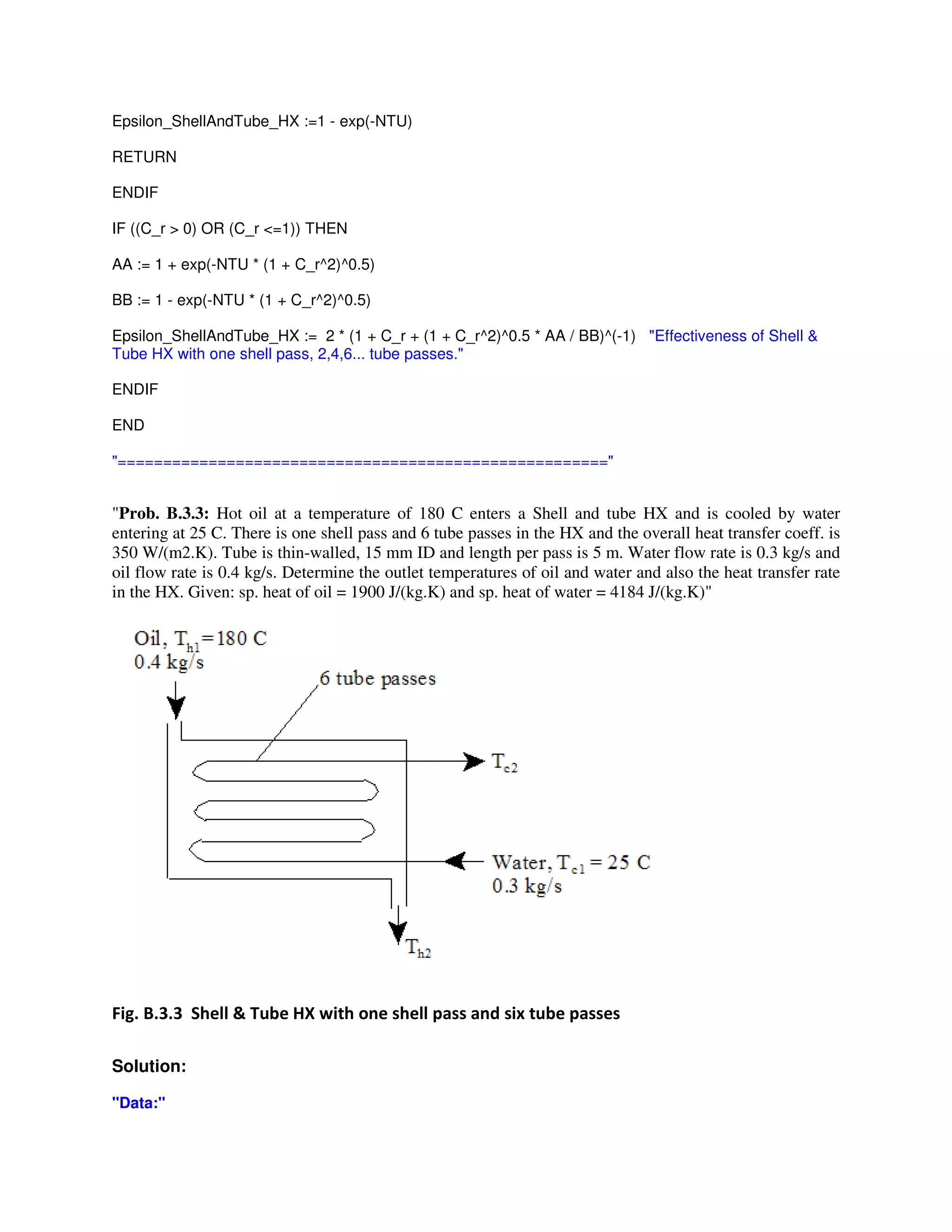
"Prob.B.3.4. A cross-flow HX (both fluids unmixed), having a heat transfer area of 8.4 m^2, is to heat air
(cp = 1005 J/kg.K) with water (cp = 4180 J/kg.K). Air enters at 18 C with a mass flow rate of 2 kg/s while
water enters at 90 C with a mass flow rate of 0.25 kg/s. Overall heat transfer coeff is 250 W/m^2.K
Calculate the exit temps of the two fluids and the heat transfer rate. [VTU - July-Aug. 2004]"
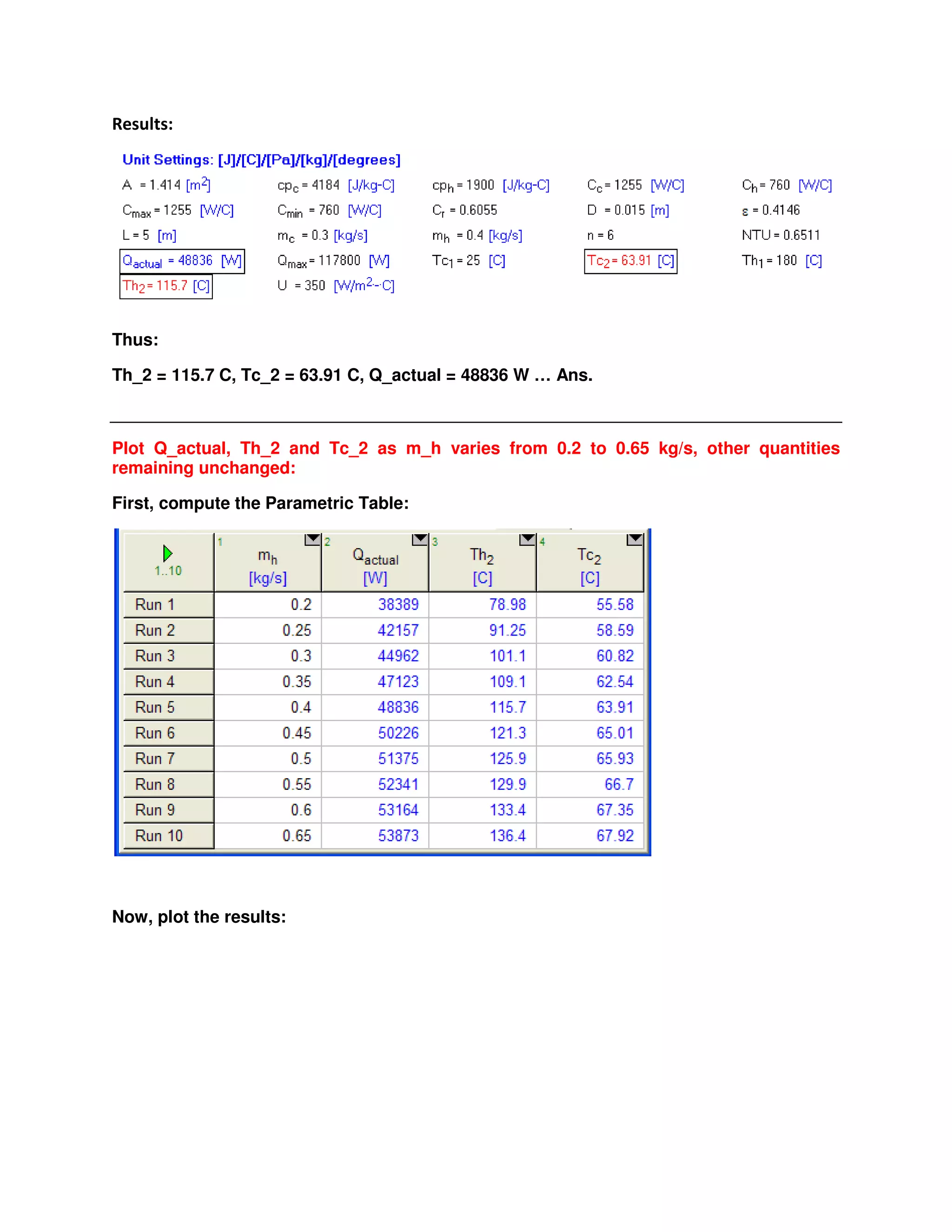
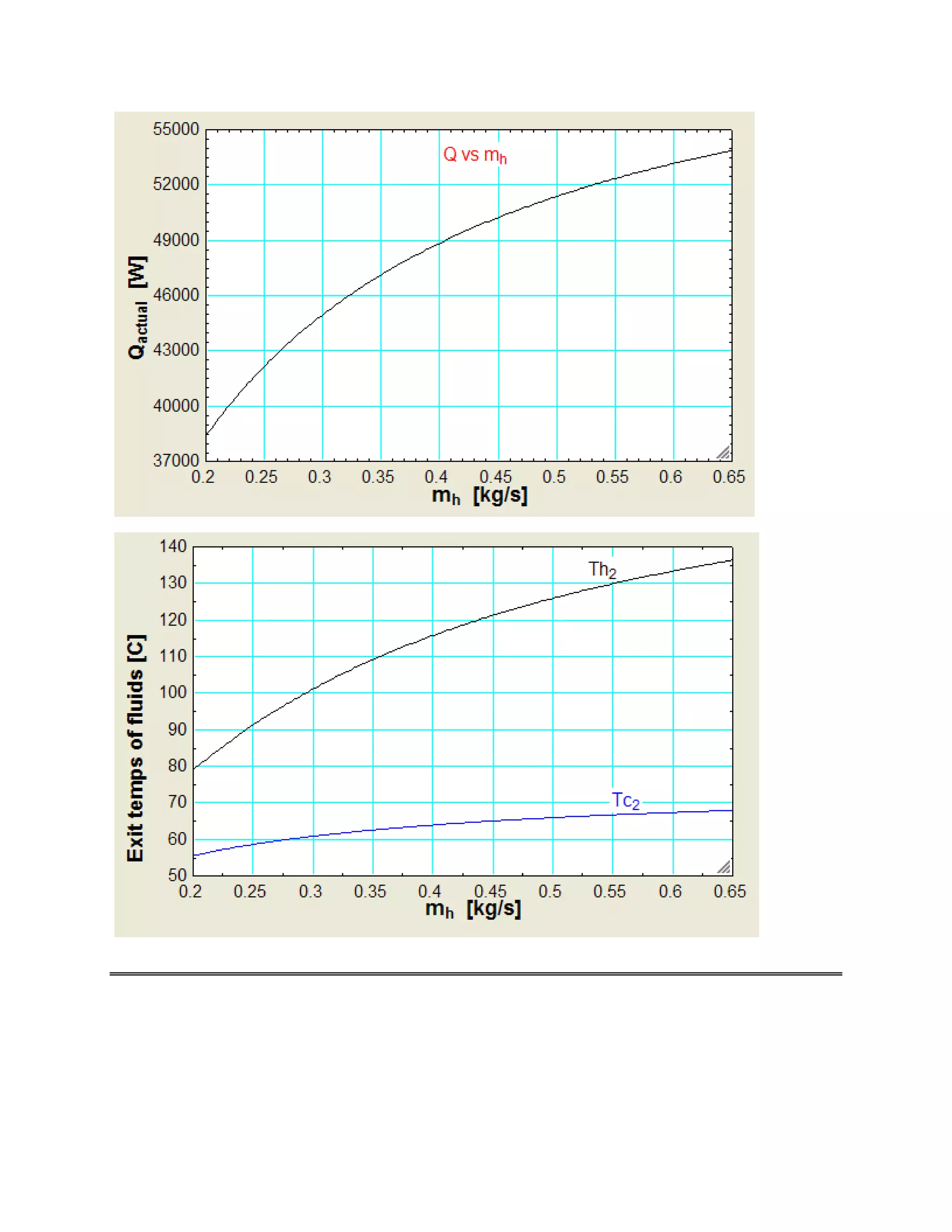
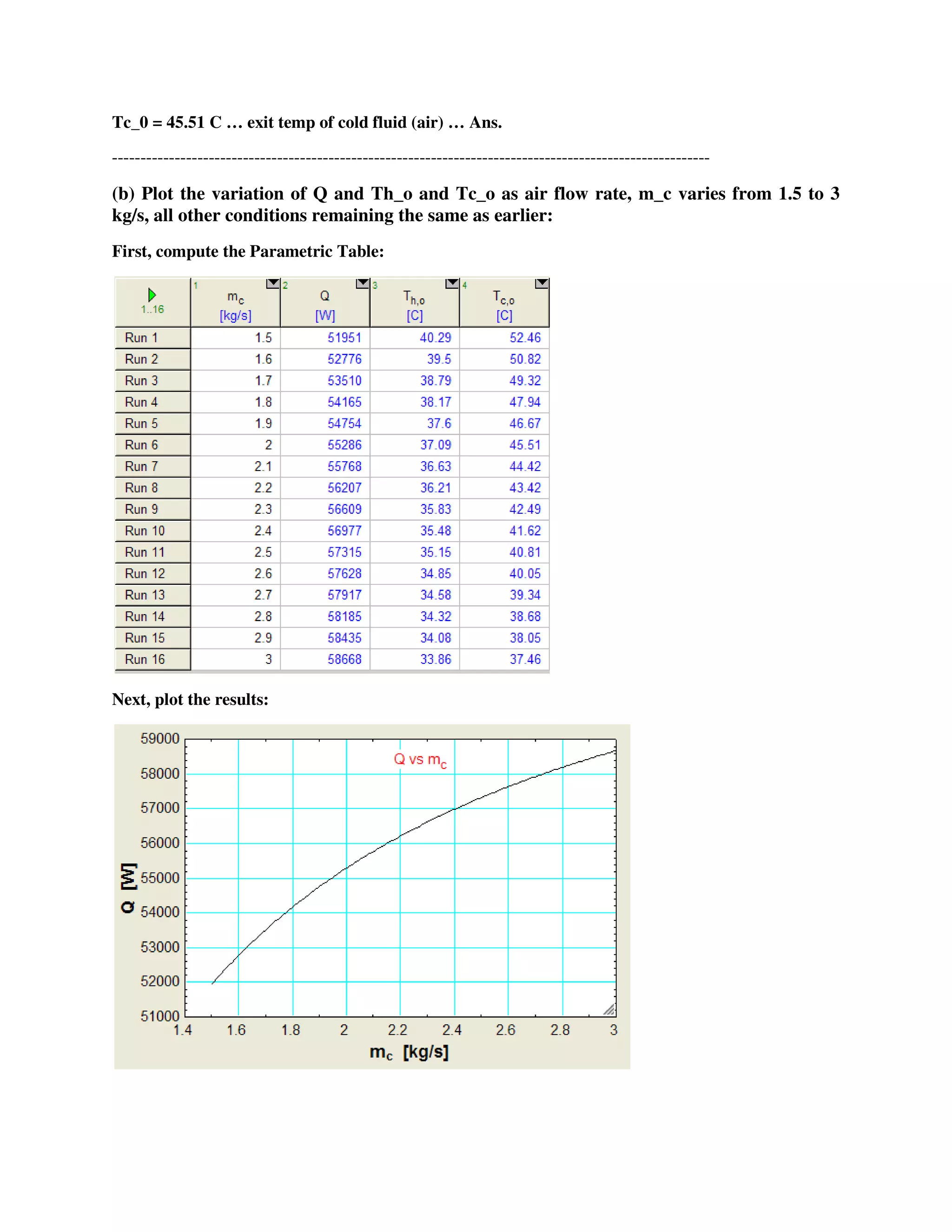
(b) Plot the variation of Q and Th_o and Tc_o as air flow rate, m_c varies from 1.5 to 3 kg/s, all other
conditions remaining the same as earlier:
Fig. Prob.B.3.4. Cross-flow arrangement

48. EES Solution:
"Data:"
m_h = 0.25 [kg/s] "....water is the hot fluid"
m_c = 2[kg/s] "....air is the cold fluid"
T_h_i = 90 [C]
T_c_i = 18 [C]
cp_c = 1005 [J/kg-C]
cp_h = 4180 [J/kg-C]
U = 250 [W/m^2-C]
A = 8.4 [m^2]
Calculations:
C_h = m_h * cp_h "W/C...= 1045 … capacity rate of hot fluid"
C_c = m_c * cp_c "W/C... = 2010 … capacity rate of cold fluid"
C_min = C_h “….min. capacity rate”
C_max = C_c ”…max. capacity rate”
C_r = C_min/C_max “… Capacity ratio”
NTU = U * A /C_min “…NTU by definition”
"For cross-flow HX: Using the EES Function for effectiveness of Cross flow HX, with both fluids Unmixed,
written earlier:"
epsilon = Epsilon_Crossflow_bothUnmixed(NTU,C_r) "Effectiveness of Cross-flow HX ..Ref: Incropera. "
"Also:"
epsilon = (T_h_i - T_h_o)/(T_h_i - T_c_i) "...determines exit temp of hot fluid, i.e. water, T_h_o"
Q= m_h * cp_h * (T_h_i - T_h_o) "W ... determines Q"
Q = m_c * cp_c * (T_c_o - T_c_i) "W...determines exit temp of cold fluid, i.e. air, T_c_o."
"====================================================================="
Results:
Thus:
Q = 55286 W … heat transferred … Ans.
Th_0 = 37.09 C … exit temp of hot fluid (water) …. Ans.

49. Tc_0 = 45.51 C … exit temp of cold fluid (air) … Ans.
---------------------------------------------------------------------------------------------------------
(b) Plot the variation of Q and Th_o and Tc_o as air flow rate, m_c varies from 1.5 to 3
kg/s, all other conditions remaining the same as earlier:
First, compute the Parametric Table:
Next, plot the results:

50. =====================================================================
# 5 L, #
MH #N, # # M #N"
FUNCTION Epsilon_Crossflow_OneUnmixed(NTU,C_mixed, C_unmixed)
"Finds the effectiveness of Crossflow HX with one fluid 'Unmixed', and the other, 'mixed':
Input: NTU, Capacity rates, C_mixed and C_unmixed .
Output: Effectiveness"
IF (C_mixed > C_unmixed ) THEN
C_r := C_unmixed / C_mixed
IF (C_r = 0) THEN
Epsilon_Crossflow_OneUnmixed := 1 - exp (-NTU)
RETURN
ENDIF
AA := -C_r * (1 - exp(-NTU))
BB = 1 - exp(AA)
Epsilon_Crossflow_OneUnmixed := (1/ C_r) * BB
ENDIF
IF (C_unmixed >= C_mixed ) THEN

51. C_r := C_mixed / C_unmixed
IF (C_r = 0) THEN
Epsilon_Crossflow_OneUnmixed := 1 - exp (-NTU)
RETURN
ENDIF
AA := (-1/C_r) * ( 1 - exp(-NTU * C_r))
Epsilon_Crossflow_OneUnmixed := 1 - exp( AA) "Effectiveness of Cross-flow HX ..Ref: Incropera. "
ENDIF
END
"======================================================"
Now, solve a problem using the above EES Function:
Prob. B.3.5. Consider a cross flow HX where oil flowing through the tubes is heated by steam flowing
across the tubes. Oil (cp = 1900 J/kg.C) is heated from 15 C to 85 C and steam (cp = 1860 J/kg.C) enters
at 130 C and leaves at 110 C with a mass flow rate of 5.2 kg/s. Overall heat transfer coeff U = 275
W/m^2.C. Calculate the surface area required for this HX.

52. EES Solution:
"Data:"
"Steam is the 'mixed' fluid and oil is the 'un-mixed' fluid."
m_h = 5.2 [kg/s] "....steam is the hot fluid, 'mixed' fluid"
T_h_i = 130 [C]
T_c_i = 15 [C]
T_c_0 = 85 [C]
T_h_0 = 110 [C]
cp_c = 1900 [J/kg-C]
cp_h = 1860 [J/kg-C]
U = 275 [W/m^2-C]
"Calculations:"
C_mixed = m_h * cp_h "W/C...= 9672 capacity rate of hot fluid"
Q = C_mixed * (T_h_i - T_h_0) "W ... heat transfer in HX"
Q = C_unmixed * (T_c_0 - T_c_i) "...finds C_unmixed, ... 2763 [W/C]"
C_unmixed = m_c * cp_c "...finds m_c, flow rate of cold fluid (oil), kg/s"
"Since we find that oil is the minimum fluid, we can write for Effectiveness:"
epsilon = (T_c_0 - T_c_i) / (T_h_i - T_c_i) "... effectivenes, by definition"
"Then, to find NTU: Use the EES Function written above for Effectiveness of this HX.
Note that when effectiveness and Capacity rates are known, the same Function determines the
other unknown, viz. NTU:"
epsilon = Epsilon_Crossflow_OneUnmixed(NTU,C_mixed, C_unmixed) "Effectiveness of Cross-flow HX
.....finds NTU "
"Also, since oil is the 'minimum' fluid:"
NTU = U * A / C_unmixed "...finds A [m^2]"
"====================================================================="

53. Results:
Thus:
Effectiveness of HX = epsilon = 0.6087 … Ans.
NTU = 1.105 …. Ans.
Q = 193440 W …. Ans.
Area of HX = A = 11.1 m^2 … Ans.
# 5 B4 B6 #
$ L"
Kays and London have studied a large number of compact heat exchanger matrices and
presented their experimental results in the form of generalized graphs. Heat transfer data is
plotted as Colburn j-factor, jH = St.Pr2/3
against Re,
where, St = Stanton number = h/(G.Cp), Pr = Prandtl number = µ.Cp/k, and
Re = G.Dh/µ, G = mass velocity (= mass flow rate/Area of cross-section), kg/(s.m2
.)
In the same graphs, friction factor, f, is also plotted against Re.
One typical graph of characteristics for a plate– finned circular tube matrix (data of Trane Co.) given
by Kays and London is shown below:

54. ( # $ 4 #
In the above graph, Reynolds No. is shown on the x-axis.
Colburn j-factor, jH is used to get heat transfer coeff. h.
Friction factor is used to get the frictional pressure drop:
Writing EES Procedure to get j_H and f for given Reynolds No. (Re):
The procedure is as follows:
Digitize the graphs for jH and f, using PlotDigitizer, a freely available, java based software.
(Ref: http://plotdigitizer.sourceforge.net).
Copy the data generated in to EXCEL, draw the curves and get curve-fit equations in EXCEL:
And, then using the curve-fit equations, write the EES Functions for j_H and f:
From EXCEL:

56. Thus, we have the curve fit equations for j_H and f:
Now, write the EES Procedure to get j_H and f:
"EES Procedure to determine Colburn j-factor (j_H) and friction factor (f) for a compact HX -
a plate- finned circular tube matrix (data of Trane Co.) given by Kays and London:"
PROCEDURE Colburn_jH_and_friction_factor(Re:j_H, f)
"Finds the Colburn j-factor (j_H) and friction factor (f) for a compact HX -
a plate- finned circular tube matrix (data of Trane Co.)
Input: Reynolds No. (Re)
Output: j_H and f"
"Remember: j_H ( = St. Pr^(2/3)) where St = (h / G. Cp), Pr = (mu . Cp / k), Re = (G. Dh / mu)"
IF ((Re < 2000) OR (Re > 12000)) THEN
CALL ERROR ('Re should be between 2000 and 12000 !')
ENDIF
Re_modified := Re / 1000

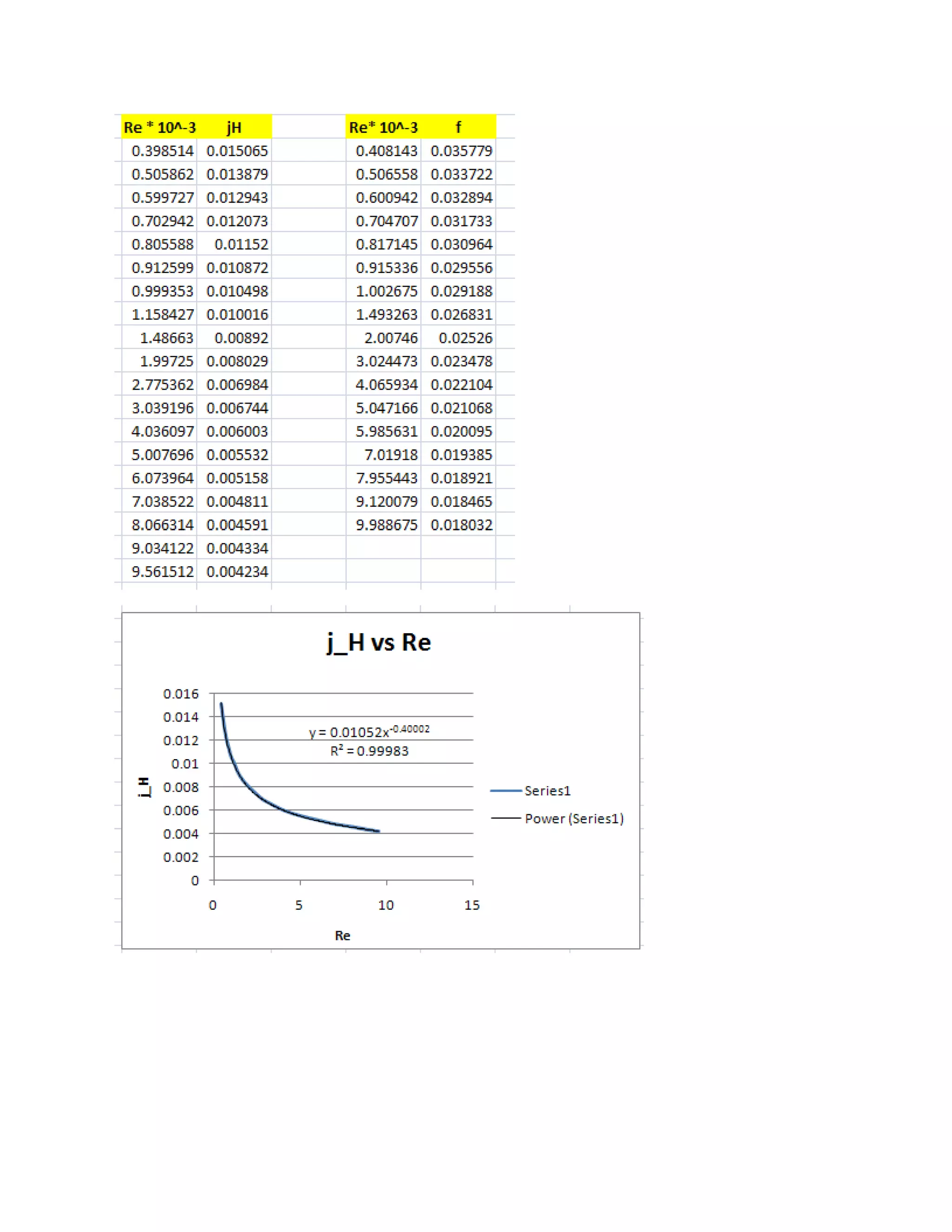
57. j_H := 0.01052 * (Re_modified)^(-0.40002)
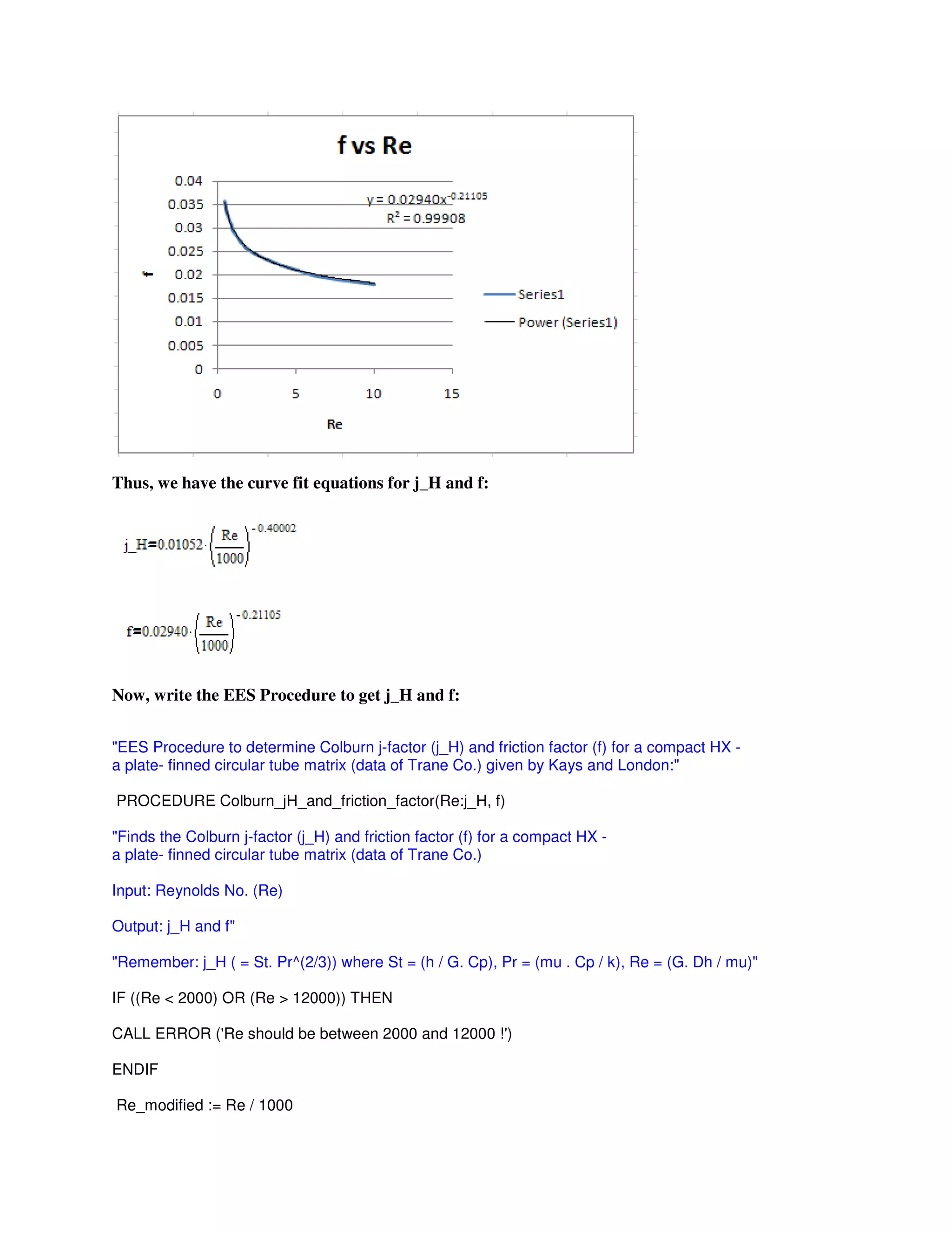
f := 0.02940 * (Re_modified)^(-0.21105)
END
"======================================================"
Now, let us solve a problem on compact heat exchangers:
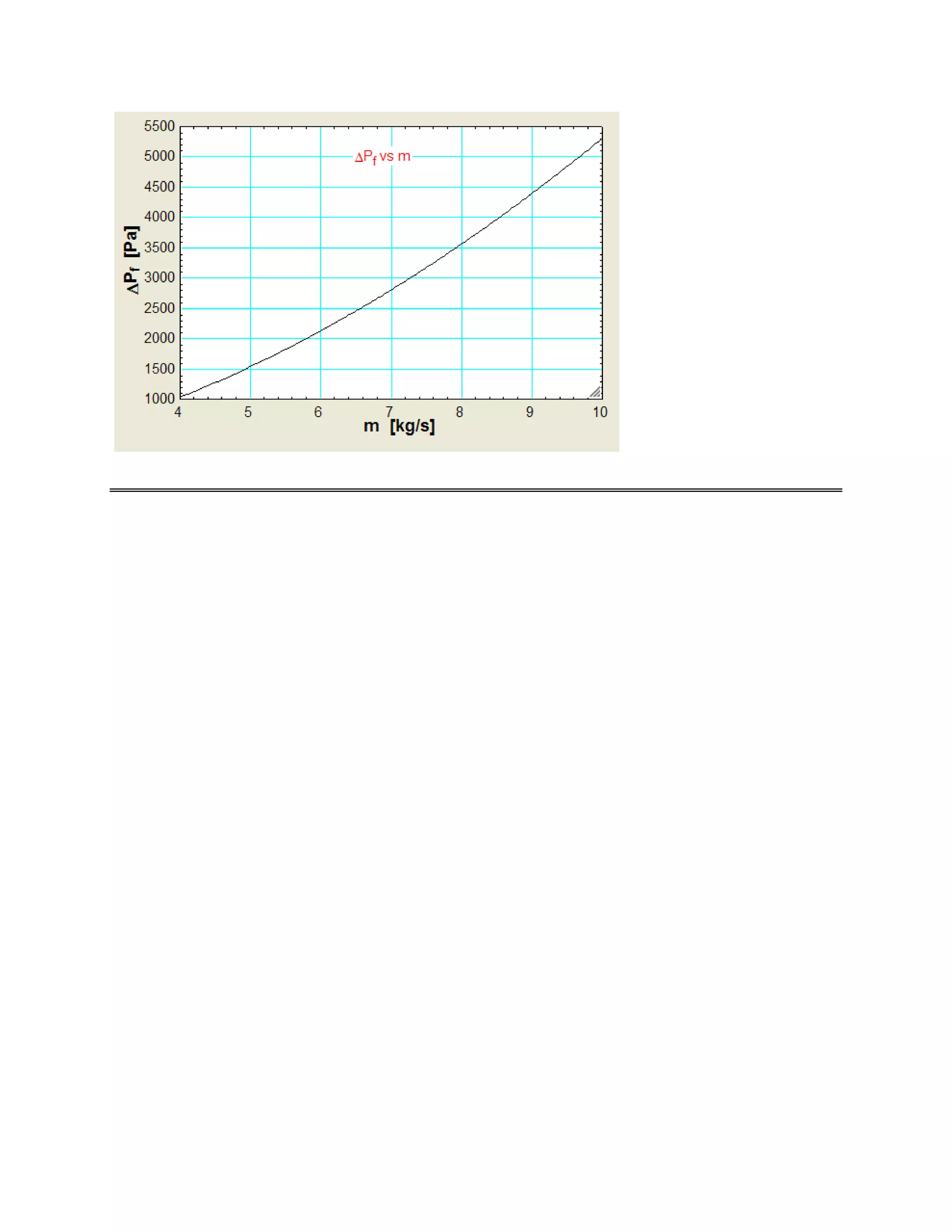
Prob. B.3.6: Air at 2 atm and 400 K flows at a rate of 5 kg/s, across a finned circular tube matrix, for
which heat transfer and friction factor characteristics are shown in Fig.1 above. Dimensions of the heat
exchanger matrix are: 1 m (W) x 0.6 m (Deep) x 0.5 m (H), as shown in Fig.below. Find: (a) the heat
transfer coeff. (b) the friction factor, and (c) ratio of core friction pressure drop to the inlet pressure.
EES Solution:
"Data:"
m = 5 [kg/s]
A_fr = 0.5 [m^2] "...frontal area"
L = 0.6 [m] "...length of flow"
P_air = 2 * 101.3 * 10^3 [Pa]
T_air = 400 - 273 "[C]"
"Properties of Air at 2 atm and 400 K:"
rho = Density(Air,T=T_air,P=P_air) "[kg/m^3]"
mu = Viscosity(Air,T=T_air)" Dyn. viscosity, kg/m.s"
cp = SpecHeat(Air,T=T_air) "sp. heat, J/kg.C"
Pr = Prandtl(Air,T=T_air) "Prandtl No."

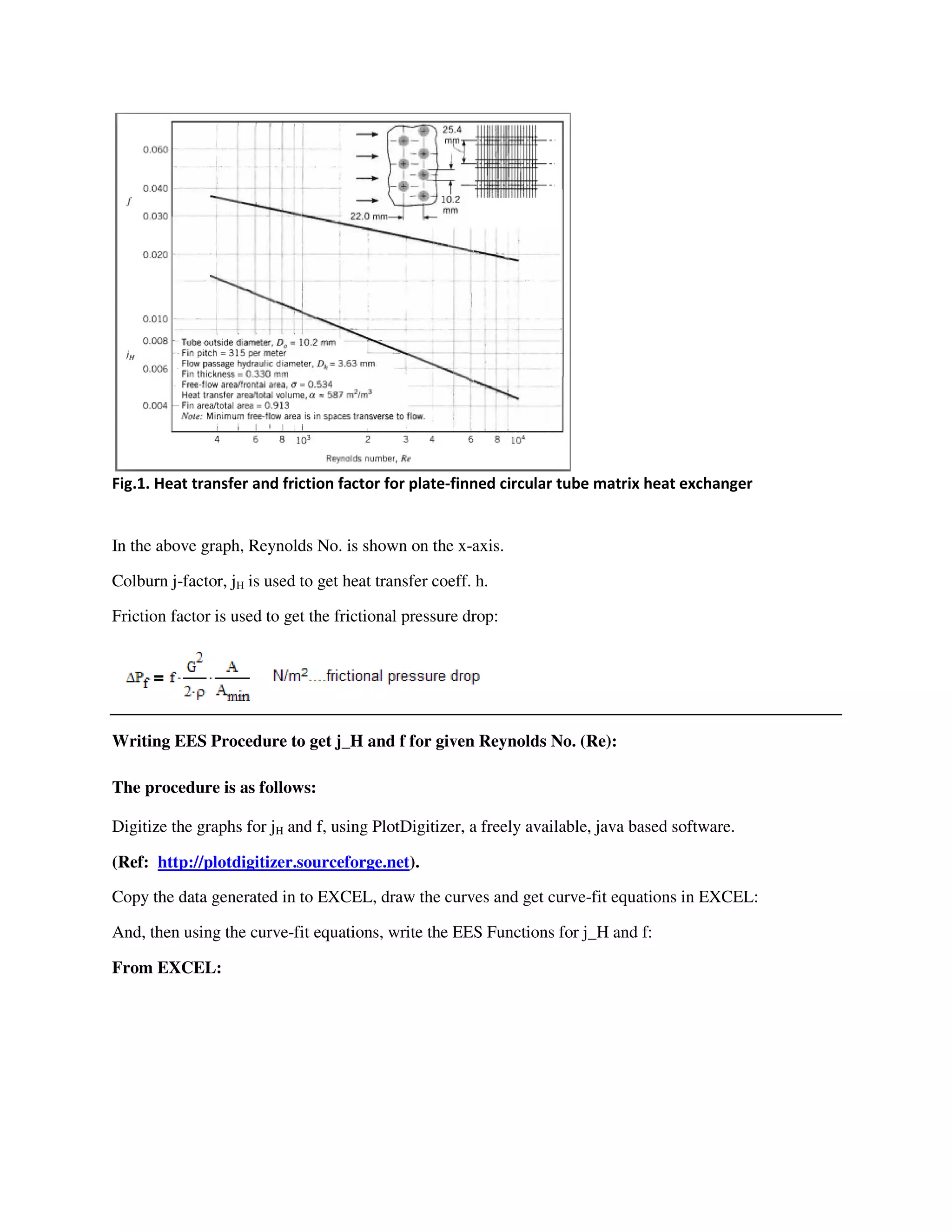
58. "From the Fig.1, i.e. Heat transfer and friction factor characteristics for plate-finned circular tube matrix
heat exchanger, we have:"
sigma = 0.534 ; D_h = 3.63E-03 "m .... hydraulic dia"
sigma = A_min / A_fr " .. by definition"
"Mass velocity: G:"
G = m / A_min " .... mass velocity, [kg/s-m^2]"
"Reynolds No.:"
Re = G * D_h / mu "...Reynolds No."
"We get Re = 2965. Now, use the EES Procedure written above to get j_H and f:"
CALL Colburn_jH_and_friction_factor(Re:j_H, f)
"But, we have:"
j_H = St * Pr^(2/3) "... Colburn j-factor"
St = h /(G * cp)"... Stanton No... h = heat tr coeff. .... finds h"
"Pressure drop:"
" DELTAP_f = f * (G^2 / (2 * rho)) * (A / A_min)
And, (A / A_min) = 4 * L / D_h . Therefore:"
DELTAP_f = f * (G^2 / (2 * rho)) * (4 * L / D_h ) " Pressure drop, N/m^2"
PressureDrop_fraction =( DELTAP_f / P_air) *100 " % . of inlet pressure"
"================================================================"
Results:

59. Thus:
(a) heat transfer coeff. = h = 162.8 W/m^2.C … Ans.
(b) friction factor = f = 0.02337 …. Ans.
(c) ratio of core friction pressure drop to the inlet pressure = 0.7582 % …. Ans.
Plot the variation of h and Pf as mass flow rate varies from 4 to 10 kg/s, other quantities
remaining unchanged:
First, compute the Parametric Table:
Now, plot the results: