Download as PDF, PPTX
![D Nagesh Kumar, IISc Optimization Methods: M2L17
Functions of a single variable
Consider the function f(x) defined for
To find the value of x* such that x* maximizes f(x) we need
to solve a single-variable optimization problem.
We have the following theorems to understand the necessary and
sufficient conditions for the relative maximum of a function of a
single variable.
a x b≤ ≤
[ , ]a b∈](https://image.slidesharecdn.com/numericalanalysisstationaryvariables-140806050354-phpapp01/85/Numerical-analysis-stationary-variables-7-320.jpg)
![D Nagesh Kumar, IISc Optimization Methods: M2L18
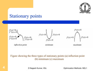
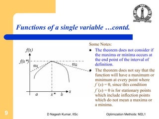
Functions of a single variable …contd.
Necessary condition : For a single variable function f(x) defined for x
which has a relative maximum at x = x* , x* if the
derivative f ‘(x) = df(x)/dx exists as a finite number at x = x* then
f ‘(x*) = 0.
We need to keep in mind that the above theorem holds good for
relative minimum as well.
The theorem only considers a domain where the function is
continuous and derivative.
It does not indicate the outcome if a maxima or minima exists at a
point where the derivative fails to exist. This scenario is shown in the
figure below, where the slopes m1 and m2 at the point of a maxima are
unequal, hence cannot be found as depicted by the theorem.
[ , ]a b∈ [ , ]a b∈](https://image.slidesharecdn.com/numericalanalysisstationaryvariables-140806050354-phpapp01/85/Numerical-analysis-stationary-variables-8-320.jpg)
![D Nagesh Kumar, IISc Optimization Methods: M2L119
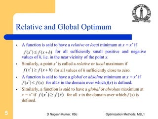
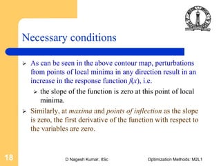
Necessary conditions …contd.
Which gives us at the stationary points. i.e. the
gradient vector of f(X), at X = X* = [x1 , x2] defined as follows,
must equal zero:
This is the necessary condition.
1 2
0; 0
f f
x x
∂ ∂
= =
∂ ∂
1
2
( *)
0
( *)
x
f
x
f
f
x
∂⎡ ⎤
Χ⎢ ⎥∂
⎢ ⎥Δ = =
∂⎢ ⎥
Χ⎢ ⎥∂⎣ ⎦
x fΔ](https://image.slidesharecdn.com/numericalanalysisstationaryvariables-140806050354-phpapp01/85/Numerical-analysis-stationary-variables-19-320.jpg)
![D Nagesh Kumar, IISc Optimization Methods: M2L120
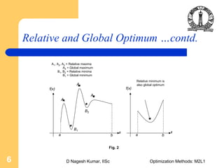
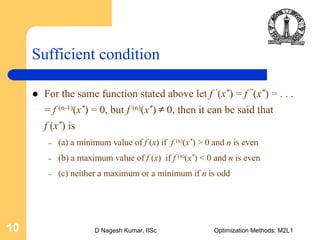
Sufficient conditions
Consider the following second order derivatives:
The Hessian matrix defined by H is made using the above second
order derivatives.
2 2 2
2 2
1 2 1 2
; ;
f f f
x x x x
∂ ∂ ∂
∂ ∂ ∂ ∂
1 2
2 2
2
1 1 2
2 2
2
1 2 2 [ , ]x x
f f
x x x
f f
x x x
⎛ ⎞∂ ∂
⎜ ⎟
∂ ∂ ∂⎜ ⎟=
⎜ ⎟∂ ∂
⎜ ⎟⎜ ⎟∂ ∂ ∂⎝ ⎠
H](https://image.slidesharecdn.com/numericalanalysisstationaryvariables-140806050354-phpapp01/85/Numerical-analysis-stationary-variables-20-320.jpg)
![D Nagesh Kumar, IISc Optimization Methods: M2L121
Sufficient conditions …contd.
The value of determinant of the H is calculated and
if H is positive definite then the point X = [x1, x2] is a
point of local minima.
if H is negative definite then the point X = [x1, x2] is a
point of local maxima.
if H is neither then the point X = [x1, x2] is neither a
point of maxima nor minima.](https://image.slidesharecdn.com/numericalanalysisstationaryvariables-140806050354-phpapp01/85/Numerical-analysis-stationary-variables-21-320.jpg)
![D Nagesh Kumar, IISc Optimization Methods: M2L123
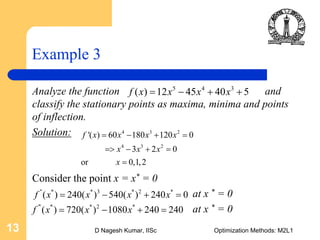
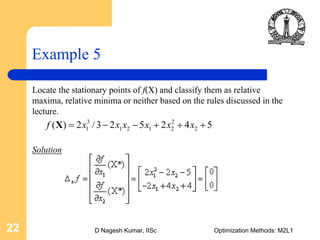
Example 5 …contd.
From ,
So the two stationary points are
X1 = [-1,-3/2] and X2 = [3/2,-1/4]
1
(X) 0
f
x
∂
=
∂
2
2 28 14 3 0x x+ + =
2 2(2 3)(4 1) 0x x+ + =
2 23/ 2 or 1/ 4x x= − = −](https://image.slidesharecdn.com/numericalanalysisstationaryvariables-140806050354-phpapp01/85/Numerical-analysis-stationary-variables-23-320.jpg)
![D Nagesh Kumar, IISc Optimization Methods: M2L124
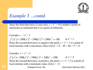
Example 5 …contd.
The Hessian of f(X) is
At X1 = [-1,-3/2] ,
2 2 2 2
12 2
1 2 1 2 2 1
4 ; 4; 2
f f f f
x
x x x x x x
∂ ∂ ∂ ∂
= = = = −
∂ ∂ ∂ ∂ ∂ ∂
14 2
2 4
x −⎡ ⎤
= ⎢ ⎥−⎣ ⎦
H
14 2
2 4
xλ
λ
λ
−
=
−
I - H
4 2
( 4)( 4) 4 0
2 4
λ
λ λ λ
λ
+
= = + − − =
−
I - H
2
16 4 0λ − − =
1 212 12λ λ= + = −
Since one eigen value is positive
and one negative, X1 is neither
a relative maximum nor a
relative minimum](https://image.slidesharecdn.com/numericalanalysisstationaryvariables-140806050354-phpapp01/85/Numerical-analysis-stationary-variables-24-320.jpg)
![D Nagesh Kumar, IISc Optimization Methods: M2L125
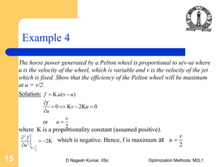
Example 5 …contd.
At X2 = [3/2,-1/4]
Since both the eigen values are positive, X-2 is a local minimum.
Minimum value of f(x) is -0.375
6 2
( 6)( 4) 4 0
2 4
λ
λ λ λ
λ
−
= = − − − =
−
I - H
1 25 5 5 5λ λ= + = −](https://image.slidesharecdn.com/numericalanalysisstationaryvariables-140806050354-phpapp01/85/Numerical-analysis-stationary-variables-25-320.jpg)
![D Nagesh Kumar, IISc Optimization Methods: M2L126
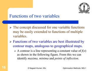
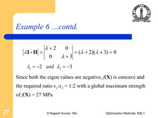
Example 6
Maximize f(X) =
;
2 2
1 1 2 220 2 6 3 / 2x x x x+ − + −
1 1
2
2
( *)
2 2 0
6 3 0
( *)
x
f
x x
f
xf
x
∂⎡ ⎤
Χ⎢ ⎥∂ −⎡ ⎤ ⎡ ⎤⎢ ⎥Δ = = =⎢ ⎥ ⎢ ⎥−∂⎢ ⎥ ⎣ ⎦⎣ ⎦Χ⎢ ⎥∂⎣ ⎦
X* = [1,2]
2 2 2
2 2
1 2 1 2
2; 3; 0
f f f
x x x x
∂ ∂ ∂
= − = − =
∂ ∂ ∂ ∂
2 0
0 3
−⎡ ⎤
= ⎢ ⎥−⎣ ⎦
H](https://image.slidesharecdn.com/numericalanalysisstationaryvariables-140806050354-phpapp01/85/Numerical-analysis-stationary-variables-26-320.jpg)


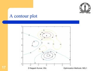
This document discusses optimization methods for functions of single and two variables. It defines stationary points as points where the derivative of a function is equal to zero. For a function of a single variable, a necessary condition for a relative maximum is that the derivative is equal to zero at that point. The sufficient condition depends on higher order derivatives. For functions of two variables, the gradient vector must be equal to zero at stationary points. The Hessian matrix formed from second order derivatives is used to classify stationary points as maxima, minima or neither. Several examples are provided to demonstrate finding stationary points and classifying them.