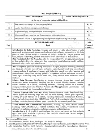
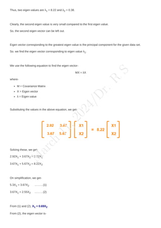
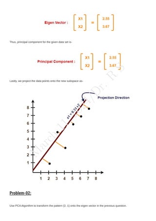
The document provides information about the syllabus for the Data Analytics (KIT-601) course. It includes 5 units that will be covered: Introduction to Data Analytics, Data Analysis techniques including regression modeling and multivariate analysis, Mining Data Streams, Frequent Itemsets and Clustering, and Frameworks and Visualization. It lists the course outcomes and Bloom's taxonomy levels. It also provides details on the topics to be covered in each unit, including proposed lecture hours, textbooks, and an evaluation scheme. The syllabus aims to discuss concepts of data analytics and apply techniques such as classification, regression, clustering, and frequent pattern mining on data.
IDENTIFICATION OF OUTLIERS IN OXAZOLINES AND OXAZOLES HIGH DIMENSION MOLECULA...IJDKP
This document summarizes an algorithm called Principal Component Outlier Detection (PrCmpOut) for identifying outliers in high-dimensional molecular descriptor datasets. PrCmpOut uses principal component analysis to transform the data into a lower-dimensional space, where it can more efficiently detect outliers using robust estimators of location and covariance. The properties of PrCmpOut are analyzed and compared to other robust outlier detection methods through simulation studies using a dataset of oxazoline and oxazole molecular descriptors. Numerical results show PrCmpOut performs well at outlier detection in high-dimensional data.
An Influence of Measurement Scale of Predictor Variable on Logistic Regressio...IJECEIAES
Much real world decision making is based on binary categories of information that agree or disagree, accept or reject, succeed or fail and so on. Information of this category is the output of a classification method that is the domain of statistical field studies (eg Logistic Regression method) and machine learning (eg Learning Vector Quantization (LVQ)). The input argument of a classification method has a very crucial role to the resulting output condition. This paper investigated the influence of various types of input data measurement (interval, ratio, and nominal) to the performance of logistic regression method and LVQ in classifying an object. Logistic regression modeling is done in several stages until a model that meets the suitability model test is obtained. Modeling on LVQ was tested on several codebook sizes and selected the most optimal LVQ model. The best model of each method compared to its performance on object classification based on Hit Ratio indicator. In logistic regression model obtained 2 models that meet the model suitability test is a model with predictive variables scaled interval and nominal, while in LVQ modeling obtained 3 pieces of the most optimal model with a different codebook. In the data with interval-scale predictor variable, the performance of both methods is the same. The performance of both models is just as bad when the data have the predictor variables of the nominal scale. In the data with predictor variable has ratio scale, the LVQ method able to produce moderate enough performance, while on logistic regression modeling is not obtained the model that meet model suitability test. Thus if the input dataset has interval or ratio-scale predictor variables than it is preferable to use the LVQ method for modeling the object classification.
Statistical inference is a process of making conclusions about a population based on a sample of data. It involves using statistical methods to draw inferences about the population parameters based on sample data. There are two main types of statistical inference: estimation and hypothesis testing. Estimation involves using sample data to estimate population parameter values like the mean or standard deviation, while hypothesis testing involves specifying and testing hypotheses about population parameters.
#Data science is a field that involves using statistical and computational methods to analyze and extract insights from data. It plays a crucial role in various industries, from business and healthcare to finance and technology.
Exploratory Data Analysis.pptx for Data Analyticsharshrnotaria
Exploratory Data Analysis (EDA) is an initial step in the data analysis process aimed at understanding the structure, relationships, and patterns within a dataset. Through EDA, analysts employ techniques like summary statistics, visualization, and dimensionality reduction to uncover insights, identify anomalies, and form hypotheses. Common EDA techniques include examining summary statistics, univariate and bivariate distributions, and relationships between variables through graphical and non-graphical methods. The goals of EDA are to gain insights, detect anomalies, and generate hypotheses for further investigation.
This Presentation is on recommended system on question paper predication using machine learning techniques. We did literature survey and implement using same technique.
Regression, multivariate analysis, clustering, and predictive modeling techniques are statistical and machine learning methods for analyzing data. Regression finds relationships between variables, multivariate analysis examines multiple variables simultaneously, clustering groups similar data points, and predictive modeling predicts unknown events. These techniques are used across many fields for tasks like prediction, classification, pattern recognition, and decision making. R software can be used to perform various data analyses using these methods.
Data Analysis: Statistical Methods: Regression modelling, Multivariate Analysis - Classification: SVM & Kernel Methods - Rule Mining - Cluster Analysis, Types of Data in Cluster Analysis, Partitioning Methods, Hierarchical Methods, Density Based Methods, Grid Based Methods, Model Based Clustering Methods, Clustering High Dimensional Data - Predictive Analytics – Data analysis using R.
Regression, multivariate analysis, clustering, and predictive modeling techniques are statistical and machine learning methods for analyzing data. Regression finds relationships between variables, multivariate analysis examines multiple variables simultaneously, clustering groups similar observations, and predictive modeling predicts unknown events. These techniques are used across many fields to discover patterns, reduce dimensions, classify data, and forecast trends. R software can be used to perform various analyses including regression, clustering, and predictive modeling.
This document compares classification and regression models using the CARET package in R. Four classification algorithms are evaluated on Titanic survival data and three regression algorithms are evaluated on property liability data. For classification, random forests performed best based on the F-measure metric. For regression, gradient boosted models performed best based on RMSE. The document concludes classification can predict Titanic survivor characteristics while regression can predict property hazards.
This document provides an overview and summary of linear regression analysis theory and computing. It discusses linear regression models and the goals of regression analysis. It also introduces some key topics that will be covered in the book, including simple and multiple linear regression, model diagnosis, generalized linear models, Bayesian linear regression, and computational methods like least squares estimation. The book aims to serve as a one-semester textbook on fundamental regression analysis concepts for graduate students.
Linear Regression with R programming.pptxanshikagoel52
The document discusses linear regression and its applications. It begins with defining data mining and business analytics. It then outlines the stages of analytics and data mining processes. Linear regression is introduced as a supervised machine learning algorithm that models the relationship between a scalar dependent variable and one or more explanatory variables. Linear regression can be used for prediction and forecasting based on fitting a model to observed data. An example case study is given of using linear regression to analyze computer price data and predict the price of a new computer configuration based on factors like CPU speed, hard drive size, RAM, etc.
Influence over the Dimensionality Reduction and Clustering for Air Quality Me...IJAEMSJORNAL
The current trend in the industry is to analyze large data sets and apply data mining, machine learning techniques to identify a pattern. But the challenges with huge data sets are the high dimensions associated with it. Sometimes in data analytics applications, large amounts of data produce worse performance. Also, most of the data mining algorithms are implemented column wise and too many columns restrict the performance and make it slower. Therefore, dimensionality reduction is an important step in data analysis. Dimensionality reduction is a technique that converts high dimensional data into much lower dimension, such that maximum variance is explained within the first few dimensions. This paper focuses on multivariate statistical and artificial neural networks techniques for data reduction. Each method has a different rationale to preserve the relationship between input parameters during analysis. Principal Component Analysis which is a multivariate technique and Self Organising Map a neural network technique is presented in this paper. Also, a hierarchical clustering approach has been applied to the reduced data set. A case study of Air quality measurement has been considered to evaluate the performance of the proposed techniques.
An application of artificial intelligent neural network and discriminant anal...Alexander Decker
This document presents a study that compares the predictive abilities of artificial neural networks and linear discriminant analysis for credit scoring. A credit dataset from a Nigerian bank with 200 applicants and 15 variables is used to build both neural network and linear discriminant models. The models are evaluated based on measures like accuracy, Wilks' lambda, and canonical correlation. Key findings are that the neural network model performs slightly better with less misclassification cost. However, variable selection is important for both models' success. Age, length of service, and other borrowing are found to be the most important predictor variables.
Anomaly detection: Core Techniques and Advances in Big Data and Deep LearningQuantUniversity
Anomaly detection (or Outlier analysis) is the identification of items, events or observations which do not conform to an expected pattern or other items in a dataset. It is used is applications such as intrusion detection, fraud detection, fault detection and monitoring processes in various domains including energy, healthcare and finance.
The document discusses data analysis and interpretation. It describes the different scales of measurement used in data analysis including nominal, ordinal, interval, and ratio scales. It also discusses various methods used for interpreting qualitative and quantitative data, such as using statistical techniques like mean and standard deviation for quantitative data. Finally, it covers different visualization techniques used in data interpretation like bar graphs, pie charts, tables, and line graphs.
Performance Comparision of Machine Learning AlgorithmsDinusha Dilanka
In this paper Compare the performance of two
classification algorithm. I t is useful to differentiate
algorithms based on computational performance rather
than classification accuracy alone. As although
classification accuracy between the algorithms is similar,
computational performance can differ significantly and it
can affect to the final results. So the objective of this paper
is to perform a comparative analysis of two machine
learning algorithms namely, K Nearest neighbor,
classification and Logistic Regression. In this paper it
was considered a large dataset of 7981 data points and 112
features. Then the performance of the above mentioned
machine learning algorithms are examined. In this paper
the processing time and accuracy of the different machine
learning techniques are being estimated by considering the
collected data set, over a 60% for train and remaining
40% for testing. The paper is organized as follows. In
Section I, introduction and background analysis of the
research is included and in section II, problem statement.
In Section III, our application and data analyze Process,
the testing environment, and the Methodology of our
analysis are being described briefly. Section IV comprises
the results of two algorithms. Finally, the paper concludes
with a discussion of future directions for research by
eliminating the problems existing with the current
research methodology.
This document discusses the different database options for handling big data: SQL, HBase, Hive, and Spark. SQL databases are not well-suited for big data due to limitations in scalability. HBase is a non-SQL database that can handle large volumes of data across clusters but lacks querying capabilities. Hive provides SQL-like querying of large datasets but is slower than other options. Spark can be used for both batch processing and interactive queries, making it a flexible option for big data workloads. The best choice depends on an application's specific needs and tradeoffs among performance, scalability, and functionality.
This document provides an overview of data analysis and graphical representation. It discusses data analytics, statistics, quantitative and qualitative data, different types of graphical representations including line graphs, bar graphs and histograms. It also covers sampling design, types of sampling including probability and non-probability sampling, and measures of central tendency such as mean, median and mode.
Data science notes for ASDS calicut 2.pptxswapnaraghav
Data science involves both statistics and practical hacking skills. It is the engineering of data - applying tools and theoretical understanding to data in a practical way. Statistical modeling is the process of using mathematical models to analyze and understand data in order to make general predictions. There are several statistical modeling techniques including linear regression, classification, resampling, non-linear models, tree-based methods, and neural networks. Unsupervised learning identifies patterns in data without pre-existing categories by techniques like clustering. Time series forecasting predicts future values based on patterns in historical time series data.
Data science uses techniques like machine learning and AI to extract meaningful insights from large, complex datasets. It relies on applied mathematics, statistics, and programming to analyze big data. Common data science tools include SAS for statistical analysis, Apache Spark for large-scale processing, BigML for machine learning modeling, Excel for visualization and basic analytics, and programming libraries like TensorFlow, Scikit-learn, and NLTK. These tools help data scientists extract knowledge and make predictions from huge amounts of data.
UNDERSTANDING LEAST ABSOLUTE VALUE IN REGRESSION-BASED DATA MININGIJDKP
This article advances our understanding of regression-based data mining by comparing the utility of Least
Absolute Value (LAV) and Least Squares (LS) regression methods. Using demographic variables from
U.S. state-wide data, we fit variable regression models to dependent variables of varying distributions
using both LS and LAV. Forecasts generated from the resulting equations are used to compare the
performance of the regression methods under different dependent variable distribution conditions. Initial
findings indicate LAV procedures better forecast in data mining applications when the dependent variable
is non-normal. Our results differ from those found in prior research using simulated data.
The document summarizes five papers that address challenges in context-aware recommendation systems using factorization methods. Three key challenges are high dimensionality, data sparsity, and cold starts. The papers propose various algorithms using matrix factorization and tensor factorization to address these challenges. COT models each context as an operation on user-item pairs to reduce dimensionality. Another approach extracts latent contexts from sensor data using deep learning and matrix factorization. CSLIM extends the SLIM algorithm to incorporate contextual ratings. TAPER uses tensor factorization to integrate various contexts for expert recommendations. Finally, GFF provides a generalized factorization framework to handle different recommendation models. The document analyzes how well each paper meets the challenges.
A Two-Step Self-Evaluation Algorithm On Imputation Approaches For Missing Cat...CSCJournals
Missing data are often encountered in data sets and a common problem for researchers in different fields of research. There are many reasons why observations may have missing values. For instance, some respondents may not report some of the items for some reason. The existence of missing data brings difficulties to the conduct of statistical analyses, especially when there is a large fraction of data which are missing. Many methods have been developed for dealing with missing data, numeric or categorical. The performances of imputation methods on missing data are key in choosing which imputation method to use. They are usually evaluated on how the missing data method performs for inference about target parameters based on a statistical model. One important parameter is the expected imputation accuracy rate, which, however, relies heavily on the assumptions of missing data type and the imputation methods. For instance, it may require that the missing data is missing completely at random. The goal of the current study was to develop a two-step algorithm to evaluate the performances of imputation methods for missing categorical data. The evaluation is based on the re-imputation accuracy rate (RIAR) introduced in the current work. A simulation study based on real data is conducted to demonstrate how the evaluation algorithm works.
This document provides a plan for processing and analyzing data for a research proposal. It discusses sorting data, performing quality checks, data processing, and analysis. The plan recommends constructing dummy tables to visualize how data will be organized before collection. It suggests sorting data after collection based on study groups for comparison. Quality checks ensure data completeness and consistency. The plan describes coding, entry, and validating data during processing. Both descriptive and analytical statistical analyses are recommended to describe patterns and explore relationships between variables. Appropriate quantitative and qualitative software are listed.
This document discusses using machine learning algorithms to predict household poverty levels. The goals are to build classification models to predict a household's poverty level as either "poor" or "non-poor" based on household attributes. Linear regression is proposed as the modeling algorithm. The document outlines collecting and preprocessing a household dataset, feature selection, model training and evaluation using metrics like MSE, RMSE and R-squared. References are provided on related work applying machine learning to poverty prediction using household surveys and satellite imagery.
Similar to IT-601 Lecture Notes-UNIT-2.pdf Data Analysis (20)
KIT-601-L-UNIT-1 (Revised) Introduction to Data Analytcs.pdfDr. Radhey Shyam
The document provides an overview of data analytics and big data concepts. It discusses the characteristics of big data, including the four V's of volume, velocity, variety and veracity. It describes different types of data like structured, semi-structured and unstructured data. The document also introduces popular big data platforms like Hadoop, Spark and Cassandra. Finally, it outlines key reasons for the need of data analytics, such as enabling better decision making and improving organizational efficiency.
SE-UNIT-3-II-Software metrics, numerical and their solutions.pdfDr. Radhey Shyam
1) The document discusses software metrics and Halstead's software science measures including program length, vocabulary, volume, difficulty, and effort. It provides the formulas to calculate these measures and an example calculation for a C function.
2) Guidelines are provided for identifying operands and operators when applying Halstead's measures to source code. Various program elements like variables, functions, and statements are classified.
3) References on software engineering and metrics are listed at the end.
Introduction to Data Analytics and data analytics life cycleDr. Radhey Shyam
The document provides an overview of data analytics and big data concepts. It discusses the characteristics of big data, including the four V's of volume, velocity, variety and veracity. It also describes different types of data like structured, semi-structured and unstructured data. The document then introduces big data platforms and tools like Hadoop, Spark and Cassandra. Finally, it discusses the need for data analytics in business, including enabling better decision making and improving efficiency.
This document provides an overview of database normalization concepts. It begins by defining normalization as the process of organizing data in a database to eliminate redundant data and ensure data dependencies are properly represented by constraints. It then discusses first normal form (1NF), which requires each cell to contain a single value. Candidate keys and super keys are also defined. The document concludes by briefly mentioning higher normal forms up to fifth normal form (5NF) and some alternative database design approaches such as NoSQL and graph databases.
This document provides an introduction to the concepts of data analytics and the data analytics lifecycle. It discusses big data in terms of the 4Vs - volume, velocity, variety and veracity. It also discusses other characteristics of big data like volatility, validity, variability and value. The document then discusses various concepts in data analytics like traditional business intelligence, data mining, statistical applications, predictive analysis, and data modeling. It explains how these concepts are used to analyze large datasets and derive value from big data. The goal of data analytics is to gain insights and a competitive advantage through analyzing large and diverse datasets.
This document is a slide presentation by Dr. Radhey Shyam on the topics of reinforcement learning and genetic algorithms. It discusses various types of applications that genetic algorithms can be used for, including control systems, design optimization, scheduling, robotics, machine learning, signal processing, game playing, and solving combinatorial optimization problems. Examples provided include gas pipeline control, missile evasion, aircraft design, manufacturing scheduling, neural network design, filter design, and solving the traveling salesman problem.
This document provides an overview of self-organizing maps (SOMs), a type of artificial neural network. It discusses the biological motivation for SOMs, which are inspired by self-organizing systems in the brain. The document outlines the basic architecture and learning algorithm of SOMs, including initialization, training procedures, and classification. It also reviews various properties of SOMs, such as their ability to approximate input spaces and perform topological ordering and density matching. Finally, applications of SOMs are briefly mentioned, such as for speech recognition, image analysis, and data visualization.
The document describes Convolutional Neural Networks (CNNs). It explains that CNNs are a type of neural network that uses convolutional layers, which apply filters to input data to extract features. This helps reduce the number of parameters needed compared to fully connected networks. The document provides examples of how CNNs can be used for image recognition, speech recognition, and text classification by applying filters that move across spatial or temporal dimensions of the input data.
1) The document discusses software metrics and Halstead's software science measures including program length, vocabulary, volume, difficulty, and effort. It provides the formulas to calculate these measures and an example calculation for a C function.
2) Guidelines are provided for identifying operands and operators when applying Halstead's measures to source code. Various program elements like variables, functions, and statements are classified.
3) The document also discusses other software metrics like lines of code (LOC) and function points which can be used to measure size and complexity. It provides a sample calculation of LOC and function points for a simple program.
The document provides an overview of Software Requirement Specification (SRS) and Software Quality Assurance (SQA). It discusses the importance of well-written requirements documents, as without them developers do not know what to build and customers do not know what to expect. The document also outlines different types of requirements like functional, non-functional, user and system requirements. It describes various requirements elicitation techniques like interviews, brainstorming sessions, use case approach etc. Finally, it discusses modeling requirements using tools like data flow diagrams, data dictionaries and entity relationship diagrams.
This document provides a 3 paragraph summary of a software engineering course titled "Software Engineering (KCS-601)" taught by Dr. Radhey Shyam at SRMCEM Lucknow. The course contents were compiled by Dr. Shyam and are available for students' academic use. Students can contact Dr. Shyam via email for any queries regarding the course material.
This document provides an overview of the unit 3 course material for Software Design taught by Dr. Radhey Shyam at SRMCEM Lucknow. The document discusses key concepts in software design including the importance of design, characteristics of good and bad design, coupling and cohesion, modularization, design models, high level design and architectural design. Specific topics covered include software design documentation, conceptual vs technical design, types of coupling and cohesion, advantages of modular systems, design frameworks, and strategies for design such as top-down, bottom-up, and hybrid approaches.
This document discusses image representation and description techniques. It begins by explaining that image segmentation results in a set of regions that need to be represented, often by their boundaries or internal characteristics, and described using features. Several boundary and regional representation and description methods are then outlined, including chain codes, shape numbers, Fourier descriptors, statistical moments, topology, and textures.
This document discusses image segmentation using morphological watersheds. It begins by explaining the concepts of regional minima, catchment basins, and watershed lines in a topographic representation of an image. It then describes the watershed algorithm which involves flooding the image from regional minima and building dams when flood waters would merge. The resulting dams represent the watershed lines and segmented boundaries. The document provides examples to illustrate the flooding process and discusses how markers can be used to limit oversegmentation from noise.
This document discusses image restoration and contains summaries of several lecture slides on image degradation and restoration models, noise models, and frequency domain filtering techniques for periodic noise reduction. It was compiled by Dr. Radhey Shyam with contributions from Dr. Philippe Cattin, and is intended for academic use by students to help explain basic concepts of image restoration.
The document is a unit on image enhancement from an image processing course. It was written by Dr. Radhey Shyam of the computer science department at BIET Lucknow, India. The unit introduces basic concepts of image enhancement in the spatial and frequency domains. Students will learn about arithmetic and logical operations on pixels to enhance images.
This document provides an overview of color image processing. It discusses that color is important for object identification and extraction. It describes the primary colors of light (red, green, blue) and pigments (cyan, magenta, yellow) and how they are used in different color models. The key color characteristics of brightness, hue, and saturation are defined. Common color models for image processing like RGB, CMY, and HSI are introduced. The RGB color model is described in more detail, representing colors as points in a color cube defined by normalized red, green, and blue values between 0 and 1.
Blood finder application project report (1).pdfKamal Acharya
Blood Finder is an emergency time app where a user can search for the blood banks as
well as the registered blood donors around Mumbai. This application also provide an
opportunity for the user of this application to become a registered donor for this user have
to enroll for the donor request from the application itself. If the admin wish to make user
a registered donor, with some of the formalities with the organization it can be done.
Specialization of this application is that the user will not have to register on sign-in for
searching the blood banks and blood donors it can be just done by installing the
application to the mobile.
The purpose of making this application is to save the user’s time for searching blood of
needed blood group during the time of the emergency.
This is an android application developed in Java and XML with the connectivity of
SQLite database. This application will provide most of basic functionality required for an
emergency time application. All the details of Blood banks and Blood donors are stored
in the database i.e. SQLite.
This application allowed the user to get all the information regarding blood banks and
blood donors such as Name, Number, Address, Blood Group, rather than searching it on
the different websites and wasting the precious time. This application is effective and
user friendly.
Null Bangalore | Pentesters Approach to AWS IAMDivyanshu
#Abstract:
- Learn more about the real-world methods for auditing AWS IAM (Identity and Access Management) as a pentester. So let us proceed with a brief discussion of IAM as well as some typical misconfigurations and their potential exploits in order to reinforce the understanding of IAM security best practices.
- Gain actionable insights into AWS IAM policies and roles, using hands on approach.
#Prerequisites:
- Basic understanding of AWS services and architecture
- Familiarity with cloud security concepts
- Experience using the AWS Management Console or AWS CLI.
- For hands on lab create account on [killercoda.com](https://killercoda.com/cloudsecurity-scenario/)
# Scenario Covered:
- Basics of IAM in AWS
- Implementing IAM Policies with Least Privilege to Manage S3 Bucket
- Objective: Create an S3 bucket with least privilege IAM policy and validate access.
- Steps:
- Create S3 bucket.
- Attach least privilege policy to IAM user.
- Validate access.
- Exploiting IAM PassRole Misconfiguration
-Allows a user to pass a specific IAM role to an AWS service (ec2), typically used for service access delegation. Then exploit PassRole Misconfiguration granting unauthorized access to sensitive resources.
- Objective: Demonstrate how a PassRole misconfiguration can grant unauthorized access.
- Steps:
- Allow user to pass IAM role to EC2.
- Exploit misconfiguration for unauthorized access.
- Access sensitive resources.
- Exploiting IAM AssumeRole Misconfiguration with Overly Permissive Role
- An overly permissive IAM role configuration can lead to privilege escalation by creating a role with administrative privileges and allow a user to assume this role.
- Objective: Show how overly permissive IAM roles can lead to privilege escalation.
- Steps:
- Create role with administrative privileges.
- Allow user to assume the role.
- Perform administrative actions.
- Differentiation between PassRole vs AssumeRole
Try at [killercoda.com](https://killercoda.com/cloudsecurity-scenario/)
Determination of Equivalent Circuit parameters and performance characteristic...pvpriya2
Includes the testing of induction motor to draw the circle diagram of induction motor with step wise procedure and calculation for the same. Also explains the working and application of Induction generator
Prediction of Electrical Energy Efficiency Using Information on Consumer's Ac...PriyankaKilaniya
Energy efficiency has been important since the latter part of the last century. The main object of this survey is to determine the energy efficiency knowledge among consumers. Two separate districts in Bangladesh are selected to conduct the survey on households and showrooms about the energy and seller also. The survey uses the data to find some regression equations from which it is easy to predict energy efficiency knowledge. The data is analyzed and calculated based on five important criteria. The initial target was to find some factors that help predict a person's energy efficiency knowledge. From the survey, it is found that the energy efficiency awareness among the people of our country is very low. Relationships between household energy use behaviors are estimated using a unique dataset of about 40 households and 20 showrooms in Bangladesh's Chapainawabganj and Bagerhat districts. Knowledge of energy consumption and energy efficiency technology options is found to be associated with household use of energy conservation practices. Household characteristics also influence household energy use behavior. Younger household cohorts are more likely to adopt energy-efficient technologies and energy conservation practices and place primary importance on energy saving for environmental reasons. Education also influences attitudes toward energy conservation in Bangladesh. Low-education households indicate they primarily save electricity for the environment while high-education households indicate they are motivated by environmental concerns.
Height and depth gauge linear metrology.pdfq30122000
Height gauges may also be used to measure the height of an object by using the underside of the scriber as the datum. The datum may be permanently fixed or the height gauge may have provision to adjust the scale, this is done by sliding the scale vertically along the body of the height gauge by turning a fine feed screw at the top of the gauge; then with the scriber set to the same level as the base, the scale can be matched to it. This adjustment allows different scribers or probes to be used, as well as adjusting for any errors in a damaged or resharpened probe.
This presentation is about Food Delivery Systems and how they are developed using the Software Development Life Cycle (SDLC) and other methods. It explains the steps involved in creating a food delivery app, from planning and designing to testing and launching. The slide also covers different tools and technologies used to make these systems work efficiently.
Build the Next Generation of Apps with the Einstein 1 Platform.
Rejoignez Philippe Ozil pour une session de workshops qui vous guidera à travers les détails de la plateforme Einstein 1, l'importance des données pour la création d'applications d'intelligence artificielle et les différents outils et technologies que Salesforce propose pour vous apporter tous les bénéfices de l'IA.
AI + Data Community Tour - Build the Next Generation of Apps with the Einstei...
IT-601 Lecture Notes-UNIT-2.pdf Data Analysis
1. M
a
r
c
h
1
1
,
2
0
2
4
/
D
r
.
R
S
Data Analytics (KIT-601)
Unit-2: Data Analysis
Dr. Radhey Shyam
Professor
Department of Information Technology
SRMCEM Lucknow
(Affiliated to Dr. A.P.J. Abdul Kalam Technical University, Lucknow)
Unit-2 has been prepared and compiled by Dr. Radhey Shyam, with grateful acknowledgment to those who
made their course contents freely available or (Contributed directly or indirectly). Feel free to use this
study material for your own academic purposes. For any query, communication can be made through this
email : shyam0058@gmail.com.
March 11, 2024
2. Data Analytics (KIT 601)
Course Outcome ( CO) Bloom’s Knowledge Level (KL)
At the end of course , the student will be able to
CO 1 Discuss various concepts of data analytics pipeline K1, K2
CO 2 Apply classification and regression techniques K3
CO 3 Explain and apply mining techniques on streaming data K2, K3
CO 4 Compare different clustering and frequent pattern mining algorithms K4
CO 5 Describe the concept of R programming and implement analytics on Big data using R. K2,K3
DETAILED SYLLABUS 3-0-0
Unit Topic Proposed
Lecture
I
Introduction to Data Analytics: Sources and nature of data, classification of data
(structured, semi-structured, unstructured), characteristics of data, introduction to Big Data
platform, need of data analytics, evolution of analytic scalability, analytic process and
tools, analysis vs reporting, modern data analytic tools, applications of data analytics.
Data Analytics Lifecycle: Need, key roles for successful analytic projects, various phases
of data analytics lifecycle – discovery, data preparation, model planning, model building,
communicating results, operationalization.
08
II
Data Analysis: Regression modeling, multivariate analysis, Bayesian modeling, inference
and Bayesian networks, support vector and kernel methods, analysis of time series: linear
systems analysis & nonlinear dynamics, rule induction, neural networks: learning and
generalisation, competitive learning, principal component analysis and neural networks,
fuzzy logic: extracting fuzzy models from data, fuzzy decision trees, stochastic search
methods.
08
III
Mining Data Streams: Introduction to streams concepts, stream data model and
architecture, stream computing, sampling data in a stream, filtering streams, counting
distinct elements in a stream, estimating moments, counting oneness in a window,
decaying window, Real-time Analytics Platform ( RTAP) applications, Case studies – real
time sentiment analysis, stock market predictions.
08
IV
Frequent Itemsets and Clustering: Mining frequent itemsets, market based modelling,
Apriori algorithm, handling large data sets in main memory, limited pass algorithm,
counting frequent itemsets in a stream, clustering techniques: hierarchical, K-means,
clustering high dimensional data, CLIQUE and ProCLUS, frequent pattern based clustering
methods, clustering in non-euclidean space, clustering for streams and parallelism.
08
V
Frame Works and Visualization: MapReduce, Hadoop, Pig, Hive, HBase, MapR,
Sharding, NoSQL Databases, S3, Hadoop Distributed File Systems, Visualization: visual
data analysis techniques, interaction techniques, systems and applications.
Introduction to R - R graphical user interfaces, data import and export, attribute and data
types, descriptive statistics, exploratory data analysis, visualization before analysis,
analytics for unstructured data.
08
Text books and References:
1. Michael Berthold, David J. Hand, Intelligent Data Analysis, Springer
2. Anand Rajaraman and Jeffrey David Ullman, Mining of Massive Datasets, Cambridge University Press.
3. John Garrett,Data Analytics for IT Networks : Developing Innovative Use Cases, Pearson Education
Curriculum & Evaluation Scheme IT & CSI (V & VI semester) 23
M
a
r
c
h
1
1
,
2
0
2
4
/
D
r
.
R
S
3. M
a
r
c
h
1
1
,
2
0
2
4
/
D
r
.
R
S
Unit-II: Data Analysis
Data analysis refers to the process of inspecting, cleaning, transforming, and modeling data
with the goal of discovering useful information, drawing conclusions, and supporting decision-
making. It is a critical component of many fields, including business, finance, healthcare, engineering, and
the social sciences.
The data analysis process typically involves the following steps:
ˆ Data collection: This step involves gathering data from various sources, such as databases, surveys,
sensors, and social media.
ˆ Data cleaning: This step involves removing errors, inconsistencies, and outliers from the data. It
may also involve imputing missing values, transforming variables, and normalizing the data.
ˆ Data exploration: This step involves visualizing and summarizing the data to gain insights and
identify patterns. This may include statistical analyses, such as descriptive statistics, correlation
analysis, and hypothesis testing.
ˆ Data modeling: This step involves developing mathematical models to predict or explain the behavior
of the data. This may include regression analysis, time series analysis, machine learning, and
other techniques.
ˆ Data visualization: This step involves creating visual representations of the data to communicate
insights and findings to stakeholders. This may include charts, graphs, tables, and other visual-
izations.
ˆ Decision-making: This step involves using the results of the data analysis to make informed deci-
sions, develop strategies, and take actions.
Data analysis is a complex and iterative process that requires expertise in statistics, programming, and
domain knowledge. It is often performed using specialized software, such as R, Python, SAS, and Excel, as
well as cloud-based platforms, such as Amazon Web Services and Google Cloud Platform. Effective data
analysis can lead to better business outcomes, improved healthcare outcomes, and a deeper understanding
of complex phenomena.
3
4. M
a
r
c
h
1
1
,
2
0
2
4
/
D
r
.
R
S
1 Regression Modeling
Regression modeling is a statistical technique used to examine the relationship between a dependent
variable (also called the outcome or response variable) and one or more independent variables (also called
predictors or explanatory variables). The goal of regression modeling is to identify the nature and strength
of the relationship between the dependent variable and the independent variable(s) and to use this infor-
mation to make predictions about the dependent variable.
There are many different types of regression models, including linear regression, logistic regression,
polynomial regression1
, and multivariate regression. Linear regression is one of the most commonly
used types of regression modeling, and it assumes that the relationship between the dependent variable and
the independent variable(s) is linear.
Regression modeling is used in a wide range of fields, including economics, finance, psychology, and
epidemiology2
, among others. It is often used to understand the relationships between different factors and
to make predictions about future outcomes.
1.1 Regression
1.1.1 Simple Linear Regression
Linear Regression— In statistics, linear regression is a linear approach to modeling the relationship
between a scalar response (or dependent variable) and one or more explanatory variables (or independent
variables). The case of one explanatory variable is called simple linear regression.
ˆ Linear regression is used to predict the continuous dependent variable using a given set of independent
variables.
ˆ Linear Regression is used for solving Regression problem.
ˆ In Linear regression, value of continuous variables are predicted.
ˆ Linear regression tried to find the best fit line, through which the output can be easily predicted.
1In statistics, polynomial regression is a form of regression analysis in which the relationship between the independent
variable x and the dependent variable y is modelled as an nth degree polynomial in x.
2Epidemiology is the study (scientific, systematic, and data-driven) of the distribution (frequency, pattern) and determinants
(causes, risk factors) of health-related states and events (not just diseases) in specified populations (neighborhood, school, city,
state, country, global)
4
5. M
a
r
c
h
1
1
,
2
0
2
4
/
D
r
.
R
S
ˆ Least square estimation method3
is used for estimation of accuracy4
.
ˆ The output for Linear Regression must be a continuous value, such as price, age, etc.
ˆ In Linear regression, it is required that relationship between dependent variable and independent
variable must be linear.
ˆ In linear regression, there may be collinearity5
between the independent variables.
Some Regression examples:
ˆ Regression analysis is used in stats to find trends in data. For example, you might guess that there is
a connection between how much you eat and how much you weigh; regression analysis can help you
quantify that.
ˆ Regression analysis will provide you with an equation for a graph so that you can make predictions
about your data. For example, if you’ve been putting on weight over the last few years, it can predict
how much you’ll weigh in ten years time if you continue to put on weight at the same rate.
ˆ It is also called simple linear regression. It establishes the relationship between two variables using
a straight line. If two or more explanatory variables have a linear relationship with the dependent
variable, the regression is called a multiple linear regression.
1.1.2 Logistic Regression
Logistic Regression— use to resolve classification problems where given an element you have to classify
the same in N categories. Typical examples are for example given a mail to classify it as spam or not, or
3The least squares method is a statistical procedure to find the best fit for a set of data points by minimizing the sum of
the offsets of points from the plotted curve. Least squares regression is used to predict the behavior of dependent variables.
4Accuracy is how close a measured value is to the actual value. Precision is how close the measured values are to each other.
5Collinearity is a condition in which some of the independent variables are highly correlated.
5
6. M
a
r
c
h
1
1
,
2
0
2
4
/
D
r
.
R
S
given a vehicle find to which category it belongs (car, truck, van, etc.). That’s basically the output is a finite
set of descrete values.
ˆ Logistic Regression is used to predict the categorical dependent variable using a given set of independent
variables.
ˆ Logistic regression is used for solving Classification problems.
ˆ In logistic Regression, we predict the values of categorical variables.
ˆ In Logistic Regression, we find the S-curve by which we can classify the samples.
ˆ Maximum likelihood estimation method is used for estimation of accuracy.
ˆ The output of Logistic Regression must be a Categorical value such as 0 or 1, Yes or No, etc.
ˆ In Logistic regression, it is not required to have the linear relationship between the dependent and
independent variable.
ˆ In logistic regression, there should not be collinearity between the independent variable.
2 Multivariate Analysis
Multivariate analysis is a statistical technique used to examine the relationships between multiple variables
simultaneously. It is used when there are multiple dependent variables and/or independent variables that
are interrelated.
Multivariate analysis is used in a wide range of fields, including social sciences, marketing, biology,
and finance, among others. There are many different types of multivariate analysis, including multivari-
ate regression, principal component analysis, factor analysis, cluster analysis, and discriminant
analysis.
6
7. M
a
r
c
h
1
1
,
2
0
2
4
/
D
r
.
R
S
Multivariate regression is similar to linear regression, but it involves more than one independent variable.
It is used to predict the value of a dependent variable based on two or more independent variables. Principal
component analysis (PCA) is a technique used to reduce the dimensionality of data by identifying patterns
and relationships between variables. Factor analysis is a technique used to identify underlying factors that
explain the correlations between multiple variables. Cluster analysis is a technique used to group objects or
individuals into clusters based on similarities or dissimilarities. Discriminant analysis is a technique used to
determine which variables discriminate between two or more groups.
Overall, multivariate analysis is a powerful tool for examining complex relationships between multiple
variables, and it can help researchers and analysts gain a deeper understanding of the data they are working
with.
3 Bayesian Modeling
Bayesian modeling is a statistical modeling approach that uses Bayesian inference to make predictions and
estimate parameters. It is named after Thomas Bayes, an 18th-century statistician who developed the Bayes
theorem, which is a key component of Bayesian modeling.
In Bayesian modeling, prior information about the parameters of interest is combined with data to
produce a posterior distribution. This posterior distribution represents the updated probability distribution
of the parameters given the data and the prior information. The posterior distribution is used to make
inferences and predictions about the parameters.
Bayesian modeling is particularly useful when there is limited data or when the data is noisy or uncertain.
It allows for the incorporation of prior knowledge and beliefs into the modeling process, which can improve
the accuracy and precision of predictions.
Bayesian modeling is used in a wide range of fields, including finance, engineering, ecology, and social
sciences. Some examples of Bayesian modeling applications include predicting stock prices, estimating the
prevalence of a disease in a population, and analyzing the effects of environmental factors on a species.
3.1 Bayes Theorem
ˆ Goal — To determine the most probable hypothesis, given the data D plus any initial knowledge
about the prior probabilities of the various hypotheses in H.
7
8. M
a
r
c
h
1
1
,
2
0
2
4
/
D
r
.
R
S
ˆ Prior probability of h, P(h) — it reflects any background knowledge we have about the chance
that h is a correct hypothesis (before having observed the data).
ˆ Prior probability of D, P(D) — it reflects the probability that training data D will be observed
given no knowledge about which hypothesis h holds.
ˆ Conditional Probability of observation D, P(D|h) — it denotes the probability of observing
data D given some world in which hypothesis h holds.
ˆ Posterior probability of h, P(h|D) — it represents the probability that h holds given the observed
training data D. It reflects our confidence that h holds after we have seen the training data D and it
is the quantity that Machine Learning researchers are interested in.
ˆ Bayes Theorem allows us to compute P(h|D) —
P(h|D) = P(D|h)P(h)/P(D)
Maximum A Posteriori (MAP) Hypothesis and Maximum Likelihood
ˆ Goal — To find the most probable hypothesis h from a set of candidate hypotheses H given the
observed data D. MAP Hypothesis,
hMAP = argmax
h∈H
P(h|D)
= argmax
h∈H
P(D|h)P(h)/P(D)
= argmax
h∈H
P(D|h)P(h)
ˆ If every hypothesis in H is equally probable a priori, we only need to consider the likelihood of the
data D given h, P(D|h). Then, hMAP becomes the Maximum Likelihood,
hML = argmax
h∈H
P(D|h)P(h)
Overall, Bayesian modeling is a powerful tool for making predictions and estimating parameters in situ-
ations where there is uncertainty and prior information is available.
8
9. M
a
r
c
h
1
1
,
2
0
2
4
/
D
r
.
R
S
4 Inference and Bayesian networks
Inference in Bayesian networks is the process of using probabilistic reasoning to make predictions or draw
conclusions about a system or phenomenon. Bayesian networks are graphical models that represent the
relationships between variables using a directed acyclic graph, where nodes represent variables and edges
represent probabilistic dependencies between the variables.
Inference in Bayesian networks involves calculating the posterior probability distribution of one or more
variables given evidence about other variables in the network. This can be done using Bayesian inference,
which involves updating the prior probability distribution of the variables using Bayes’ theorem and the
observed evidence.
The posterior distribution can be used to make predictions or draw conclusions about the system or
phenomenon being modeled. For example, in a medical diagnosis system, the posterior probability of a
particular disease given a set of symptoms can be calculated using a Bayesian network. This can help
clinicians make a more accurate diagnosis and choose appropriate treatments.
Bayesian networks and inference are widely used in many fields, including artificial intelligence, decision
making, finance, and engineering. They are particularly useful in situations where there is uncertainty and
probabilistic relationships between variables need to be modeled and analyzed.
4.1 BAYESIAN NETWORKS
ˆ Abbreviation : BBN (Bayesian Belief Network)
ˆ Synonyms: Bayes (ian) network, Bayes(ian) model, Belief network, Decision network, or probabilistic
directed acyclic graphical model.
ˆ A BBN is a probabilistic graphical model that represents a set of variables and their conditional
dependencies via a Directed Acyclic Graph (DAG).
9
10. M
a
r
c
h
1
1
,
2
0
2
4
/
D
r
.
R
S
ˆ BBNs enable us to model and reason about uncertainty. BBNs accommodate both subjective proba-
bilities and probabilities based on objective data.
ˆ The most important use of BBNs is in revising probabilities in the light of actual observations of events.
ˆ Nodes represent variables in the Bayesian sense: observable quantities, hidden variables or hypotheses.
Edges represent conditional dependencies.
ˆ Each node is associated with a probability function that takes, as input, a particular set of probabilities
for values for the node’s parent variables, and outputs the probability of the values of the variable
represented by the node.
ˆ Prior Probabilities: e.g. P(RAIN)
ˆ Conditional Probabilities: e.g. P(SPRINKLER | RAIN)
ˆ Joint Probability Function: P(GRASS WET, SPRINKLER, RAIN) = P(GRASS WET | RAIN,
SPRINKLER) * P(SPRINKLER | RAIN) * P ( RAIN)
ˆ Typically the probability functions are described in table form.
10
11. M
a
r
c
h
1
1
,
2
0
2
4
/
D
r
.
R
S
ˆ BN cannot be used to model the correlation relationships between random variables.
Overall, inference in Bayesian networks is a powerful tool for making predictions and drawing conclusions
in situations where there is uncertainty and complex probabilistic relationships between variables.
4.2 Support Vector and Kernel Methods
Support vector machines (SVMs) and kernel methods are commonly used in machine learning and pattern
recognition to solve classification and regression problems.
SVMs are a type of supervised learning algorithm that aims to find the optimal hyperplane that separates
the data into different classes. The optimal hyperplane is the one that maximizes the margin, or the distance
between the hyperplane and the closest data points from each class. SVMs can also use kernel functions to
transform the original input data into a higher dimensional space, where it may be easier to find a separating
hyperplane.
Kernel methods are a class of algorithms that use kernel functions to compute the similarity between
pairs of data points. Kernel functions can transform the input data into a higher dimensional feature space,
where linear methods can be applied more effectively. Some commonly used kernel functions include linear,
polynomial, and radial basis functions.
Kernel methods are used in a variety of applications, including image recognition, speech recognition,
11
12. M
a
r
c
h
1
1
,
2
0
2
4
/
D
r
.
R
S
and natural language processing. They are particularly useful in situations where the data is non-linear and
the relationship between variables is complex.
History of SVM6
ˆ SVM is related to statistical learning theory.
ˆ SVM was first introduced in 1992.
ˆ SVM becomes popular because of its success in handwritten digit recognition 1.1% test error rate for
SVM. This is the same as the error rates of a carefully constructed neural network.
ˆ SVM is now regarded as an important example of “kernel methods”, one of the key area in machine
learning
Binary Classification
Given training data (xi, yi) for i = 1 . . . N, with
xi ∈ Rd and yi ∈ {−1, 1}, learn a classifier f(x)
such that
f(xi)
(
≥ 0 yi = +1
< 0 yi = −1
i.e. yif(xi) > 0 for a correct classification.
Linear separability
linearly
separable
not
linearly
separable
6Support vector machine is a linear model and it always looks for a hyperplane to separate one class from another. I will
focus on two-dimensional case because it is easier to comprehend and - possible to visualize to give some intuition, however
bear in mind that this is true for higher dimensions (simply lines change into planes, parabolas into paraboloids etc.).
12
13. M
a
r
c
h
1
1
,
2
0
2
4
/
D
r
.
R
S
Linear classifiers
X2
X1
A linear classifier has the form
• in 2D the discriminant is a line
• is the normal to the line, and b the bias
• is known as the weight vector
f(x) = 0
f(x) = w>x + b
f(x) > 0
f(x) < 0
Linear classifiers
A linear classifier has the form
• in 3D the discriminant is a plane, and in nD it is a hyperplane
For a K-NN classifier it was necessary to `carry’ the training data
For a linear classifier, the training data is used to learn w and then discarded
Only w is needed for classifying new data
f(x) = 0
f(x) = w>x + b
Given linearly separable data xi labelled into two categories yi = {-1,1} ,
find a weight vector w such that the discriminant function
separates the categories for i = 1, .., N
• how can we find this separating hyperplane ?
The Perceptron Classifier
f(xi) = w>xi + b
The Perceptron Algorithm
Write classifier as
• Initialize w = 0
• Cycle though the data points { xi, yi }
• if xi is misclassified then
• Until all the data is correctly classified
w ← w + α sign(f(xi)) xi
f(xi) = w̃>x̃i + w0 = w>xi
where w = (w̃, w0), xi = (x̃i, 1)
13
14. M
a
r
c
h
1
1
,
2
0
2
4
/
D
r
.
R
S
For example in 2D
X2
X1
X2
X1
w
before update after update
w
NB after convergence w =
PN
i αixi
• Initialize w = 0
• Cycle though the data points { xi, yi }
• if xi is misclassified then
• Until all the data is correctly classified
w ← w + α sign(f(xi)) xi
xi
• if the data is linearly separable, then the algorithm will converge
• convergence can be slow …
• separating line close to training data
• we would prefer a larger margin for generalization
-15 -10 -5 0 5 10
-10
-8
-6
-4
-2
0
2
4
6
8
Perceptron
example
What is the best w?
• maximum margin solution: most stable under perturbations of the inputs
14
15. M
a
r
c
h
1
1
,
2
0
2
4
/
D
r
.
R
S
Tennis example
Humidity
Temperature
= play tennis
= do not play tennis
Linear Support Vector
Machines
x1
x2
=+1
=-1
Data: <xi,yi>, i=1,..,l
xi Rd
yi {-1,+1}
=-1
=+1
Data: <xi,yi>, i=1,..,l
xi Rd
yi {-1,+1}
All hyperplanes in Rd
are parameterize by a vector (w) and a constant b.
Can be expressed as w•x+b=0 (remember the equation for a hyperplane
from algebra!)
Our aim is to find such a hyperplane f(x)=sign(w•x+b), that
correctly classify our data.
f(x)
Linear SVM 2
15
16. M
a
r
c
h
1
1
,
2
0
2
4
/
D
r
.
R
S
d+
d-
Definitions
Define the hyperplane H such that:
xi•w+b +1 when yi =+1
xi•w+b -1 when yi =-1
d+ = the shortest distance to the closest positive point
d- = the shortest distance to the closest negative point
The margin of a separating hyperplane is d+
+ d-
.
H
H1 and H2 are the planes:
H1: xi•w+b = +1
H2: xi•w+b = -1
The points on the planes
H1 and H2 are the
Support Vectors
H1
H2
Maximizing the margin
d+
d-
We want a classifier with as big margin as possible.
Recall the distance from a point(x0,y0) to a line:
Ax+By+c = 0 is|A x0 +B y0 +c|/sqrt(A2
+B2
)
The distance between H and H1 is:
|w•x+b|/||w||=1/||w||
The distance between H1 and H2 is: 2/||w||
In order to maximize the margin, we need to minimize ||w||. With the
condition that there are no datapoints between H1 and H2:
xi•w+b +1 when yi =+1
xi•w+b -1 when yi =-1 Can be combined into yi(xi•w) 1
H1
H2
H
Constrained Optimization
Problem
0
and
0
subject to
2
1
Maximize
:
yields
g
simplifyin
and
,
into
back
ng
substituti
0,
to
them
setting
s,
derivative
the
Taking
0.
be
must
and
both
respect
with
of
derivative
partial
the
extremum,
At the
1
)
(
||
||
2
1
)
,
,
(
where
,
)
,
,
(
inf
maximize
:
method
Lagrangian
all
for
1
)
(
subject to
||
||
Minimize
,
i
i
i
i
i j
i
j
i
j
i
j
i
i
i
i
i
i
i
i
y
y
y
L
b
L
b
y
b
L
b
L
i
b
y
x
x
w
w
x
w
w
w
w
x
w
w
w
w
16
17. M
a
r
c
h
1
1
,
2
0
2
4
/
D
r
.
R
S
Quadratic Programming
• Why is this reformulation a good thing?
• The problem
is an instance of what is called a positive, semi-definite
programming problem
• For a fixed real-number accuracy, can be solved in
O(n log n) time = O(|D|2 log |D|2)
0
and
0
subject to
2
1
Maximize
,
i
i
i
i
i j
i
j
i
j
i
j
i
i
y
y
y
x
x
Problems with linear SVM
=-1
=+1
What if the decision function is not a linear?
Kernel Trick
)
2
,
,
(
space
in the
separable
linearly
are
points
Data
2
1
2
2
2
1 x
x
x
x
2
,
)
,
(
Here,
directly!
compute
easy to
often
is
:
thing
Cool
)
(
)
(
)
,
(
Define
)
(
)
(
2
1
maximize
want to
We
j
i
j
i
j
i
j
i
i j
i
j
i
j
i
j
i
i
K
K
F
F
K
F
F
y
y
x
x
x
x
x
x
x
x
x
x
17
18. M
a
r
c
h
1
1
,
2
0
2
4
/
D
r
.
R
S
Other Kernels
The polynomial kernel
K(xi,xj) = (xi•xj + 1)p
, where p is a tunable parameter.
Evaluating K only require one addition and one exponentiation
more than the original dot product.
Gaussian kernels (also called radius basis functions)
K(xi,xj) = exp(||xi-xj ||2
/22
)
Overtraining/overfitting
=-1
=+1
An example: A botanist really knowing trees.Everytime he sees a new tree,
he claims it is not a tree.
A well known problem with machine learning methods is overtraining.
This means that we have learned the training data very well, but
we can not classify unseen examples correctly.
Overtraining/overfitting 2
It can be shown that: The portion, n, of unseen data that will be
missclassified is bounded by:
n Number of support vectors / number of training examples
A measure of the risk of overtraining with SVM (there are also other
measures).
Ockham´s razor principle: Simpler system are better than more complex ones.
In SVM case: fewer support vectors mean a simpler representation of the
hyperplane.
Example: Understanding a certain cancer if it can be described by one gene
is easier than if we have to describe it with 5000.
18
19. M
a
r
c
h
1
1
,
2
0
2
4
/
D
r
.
R
S
A practical example, protein
localization
• Proteins are synthesized in the cytosol.
• Transported into different subcellular
locations where they carry out their
functions.
• Aim: To predict in what location a
certain protein will end up!!!
Overall, SVMs and kernel methods are powerful tools for solving classification and regression problems. They
can handle complex data and provide accurate predictions, making them valuable in many fields, including
finance, healthcare, and engineering.
5 Analysis of Time Series: Linear Systems Analysis & Nonlinear
Dynamics
Time series analysis is a statistical technique used to analyze time-dependent data. It involves studying the
patterns and trends in the data over time and making predictions about future values.
Linear systems analysis is a technique used in time series analysis to model the behavior of a system
using linear equations. Linear models assume that the relationship between variables is linear and that the
system is time-invariant, meaning that the relationship between variables does not change over time. Linear
systems analysis involves techniques such as autoregressive (AR) and moving average (MA) models, which
use past values of a variable to predict future values.
Nonlinear dynamics is another approach to time series analysis that considers systems that are not
described by linear equations. Nonlinear systems are often more complex and can exhibit chaotic behavior,
making them more difficult to model and predict. Nonlinear dynamics involves techniques such as chaos
theory and fractal analysis, which use mathematical concepts to describe the behavior of nonlinear systems.
Both linear systems analysis and nonlinear dynamics have applications in a wide range of fields, including
finance, economics, and engineering. Linear models are often used in situations where the data is relatively
simple and the relationship between variables is well understood. Nonlinear dynamics is often used in
19
20. M
a
r
c
h
1
1
,
2
0
2
4
/
D
r
.
R
S
situations where the data is more complex and the relationship between variables is not well understood.
There are several components of time series analysis, including:
1. Trend Analysis: Trend analysis is used to identify the long-term patterns and trends in the data. It
can be a linear or non-linear trend and may show an upward, downward or flat trend.
2. Seasonal Analysis: Seasonal analysis is used to identify the recurring patterns in the data that occur
within a fixed time period, such as a week, month, or year.
3. Cyclical Analysis: Cyclical analysis is used to identify the patterns that are not necessarily regular
or fixed in duration, but do show a tendency to repeat over time, such as economic cycles or business
cycles.
4. Irregular Analysis: Irregular analysis is used to identify any random fluctuations or noise in the
data that cannot be attributed to any of the above components.
5. Forecasting: Forecasting is the process of predicting future values of a time series based on its past
behavior. It can be done using various statistical techniques such as moving averages, exponential
smoothing, and regression analysis.
Overall, time series analysis is a powerful tool for studying time-dependent data and making predictions
about future values. Linear systems analysis and nonlinear dynamics are two approaches to time series
analysis that can be used in different situations to model and predict complex systems.
6 Rule Induction
Rule induction is a machine learning technique used to identify patterns in data and create a set of rules that
can be used to make predictions or decisions about new data. It is often used in decision tree algorithms
and can be applied to both classification and regression problems.
The rule induction process involves analyzing the data to identify common patterns and relationships
between the variables. These patterns are used to create a set of rules that can be used to classify or predict
new data. The rules are typically in the form of ”if-then” statements, where the ”if” part specifies the
conditions under which the rule applies and the ”then” part specifies the action or prediction to be taken.
Rule induction algorithms can be divided into two main types: top-down and bottom-up. Top-down
algorithms start with a general rule that applies to the entire dataset and then refine the rule based on
20
21. M
a
r
c
h
1
1
,
2
0
2
4
/
D
r
.
R
S
the data. Bottom-up algorithms start with individual data points and then group them together based on
common attributes.
Rule induction has many applications in fields such as finance, healthcare, and marketing. For example,
it can be used to identify patterns in financial data to predict stock prices or to analyze medical data to
identify risk factors for certain diseases.
Overall, rule induction is a powerful machine learning technique that can be used to identify patterns
in data and create rules that can be used to make predictions or decisions. It is a useful tool for solving
classification and regression problems and has many applications in various fields.
7 Neural Networks: Learning and Generalization
Neural networks are a class of machine learning algorithms that are inspired by the structure and function
of the human brain. They are used to learn complex patterns and relationships in data and can be used for
a variety of tasks, including classification, regression, and clustering.
Learning in neural networks refers to the process of adjusting the weights and biases of the network to
improve its performance on a particular task. This is typically done through a process called backpropagation,
which involves propagating the errors from the output layer back through the network and adjusting the
weights and biases accordingly.
Generalization in neural networks refers to the ability of the network to perform well on new, unseen
data. A network that has good generalization performance is able to accurately predict the outputs for new
inputs that were not included in the training set. Generalization performance is typically evaluated using a
separate validation set or by cross-validation.
Overfitting is a common problem in neural networks, where the network becomes too complex and starts
to fit the noise in the training data, rather than the underlying patterns. This can result in poor generalization
performance on new data. Techniques such as regularization, early stopping, and dropout are often used to
prevent overfitting and improve generalization performance.
Overall, learning and generalization are two important concepts in neural networks. Learning involves
adjusting the weights and biases of the network to improve its performance, while generalization refers
to the ability of the network to perform well on new, unseen data. Effective techniques for learning and
generalization are critical for building accurate and useful neural network models.
21
27. M
a
r
c
h
1
1
,
2
0
2
4
/
D
r
.
R
S
8 Competitive Learning
Competitive learning is a type of machine learning technique in which a set of neurons compete to be
activated by input data. The neurons are organized into a layer, and each neuron receives the same input
data. However, only one neuron is activated, and the competition is based on a set of rules that determine
which neuron is activated.
The competition in competitive learning is typically based on a measure of similarity between the input
data and the weights of each neuron. The neuron with the highest similarity to the input data is activated,
and the weights of that neuron are updated to become more similar to the input data. This process is repeated
for multiple iterations, and over time, the neurons learn to become specialized in recognizing different types
of input data.
Competitive learning is often used for unsupervised learning tasks, such as clustering or feature extraction.
In clustering, the neurons learn to group similar input data into clusters, while in feature extraction, the
neurons learn to recognize specific features in the input data.
One of the advantages of competitive learning is that it can be used to discover hidden structures and
patterns in data without the need for labeled data. This makes it particularly useful for applications such
as image and speech recognition, where labeled data can be difficult and expensive to obtain.
Overall, competitive learning is a powerful machine learning technique that can be used for a variety of
unsupervised learning tasks. It involves a set of neurons that compete to be activated by input data, and
over time, the neurons learn to become specialized in recognizing different types of input data.
27
30. M
a
r
c
h
1
1
,
2
0
2
4
/
D
r
.
R
S
9 Principal Component Analysis and Neural Networks
Principal component analysis (PCA) and neural networks are both machine learning techniques that can be
used for a variety of tasks, including data compression, feature extraction, and dimensionality reduction.
PCA is a linear technique that involves finding the principal components of a dataset, which are the
directions of greatest variance. The principal components can be used to reduce the dimensionality of the
data, while preserving as much of the original variance as possible.
Neural networks, on the other hand, are nonlinear techniques that involve multiple layers of interconnected
neurons. Neural networks can be used for a variety of tasks, including classification, regression, and clustering.
They can also be used for feature extraction, where the network learns to identify the most important features
of the input data.
PCA and neural networks can be used together for a variety of tasks. For example, PCA can be used to
reduce the dimensionality of the data before feeding it into a neural network. This can help to improve the
performance of the network by reducing the amount of noise and irrelevant information in the input data.
Neural networks can also be used to improve the performance of PCA. In some cases, PCA can be
limited by its linear nature, and may not be able to capture complex nonlinear relationships in the data. By
combining PCA with a neural network, the network can learn to capture these nonlinear relationships and
improve the accuracy of the PCA results.
Overall, PCA and neural networks are both powerful machine learning techniques that can be used for
a variety of tasks. When used together, they can improve the performance and accuracy of each technique
and help to solve more complex problems.
30
31. Pattern Recognition
Tag: Principal Component Analysis Numerical Example
Principal Component Analysis | Dimension Reduction
Dimension Reduction-
In pattern recognition, Dimension Reduction is defined as-
It is a process of converting a data set having vast dimensions into a data set with lesser dimensions.
It ensures that the converted data set conveys similar information concisely.
Example-
Consider the following example-
The following graph shows two dimensions x1 and x2.
x1 represents the measurement of several objects in cm.
x2 represents the measurement of several objects in inches.
In machine learning,
Using both these dimensions convey similar information.
Also, they introduce a lot of noise in the system.
So, it is better to use just one dimension.
Using dimension reduction techniques-
We convert the dimensions of data from 2 dimensions (x1 and x2) to 1 dimension (z1).
M
a
r
c
h
1
1
,
2
0
2
4
/
D
r
.
R
S
32. It makes the data relatively easier to explain.
Benefits-
Dimension reduction offers several benefits such as-
It compresses the data and thus reduces the storage space requirements.
It reduces the time required for computation since less dimensions require less computation.
It eliminates the redundant features.
It improves the model performance.
Dimension Reduction Techniques-
The two popular and well-known dimension reduction techniques are-
1. Principal ComponentAnalysis (PCA)
2. Fisher Linear DiscriminantAnalysis (LDA)
In this article, we will discuss about Principal ComponentAnalysis.
Principal Component Analysis-
Principal ComponentAnalysis is a well-known dimension reduction technique.
It transforms the variables into a new set of variables called as principal components.
These principal components are linear combination of original variables and are orthogonal.
M
a
r
c
h
1
1
,
2
0
2
4
/
D
r
.
R
S
33. The first principal component accounts for most of the possible variation of original data.
The second principal component does its best to capture the variance in the data.
There can be only two principal components for a two-dimensional data set.
PCA Algorithm-
The steps involved in PCAAlgorithm are as follows-
Step-01: Get data.
Step-02: Compute the mean vector (µ).
Step-03: Subtract mean from the given data.
Step-04: Calculate the covariance matrix.
Step-05: Calculate the eigen vectors and eigen values of the covariance matrix.
Step-06: Choosing components and forming a feature vector.
Step-07: Deriving the new data set.
PRACTICE PROBLEMS BASED ON PRINCIPAL COMPONENT ANALYSIS-
Problem-01:
Given data = { 2, 3, 4, 5, 6, 7 ; 1, 5, 3, 6, 7, 8 }.
Compute the principal component using PCAAlgorithm.
OR
Consider the two dimensional patterns (2, 1), (3, 5), (4, 3), (5, 6), (6, 7), (7, 8).
Compute the principal component using PCAAlgorithm.
OR
M
a
r
c
h
1
1
,
2
0
2
4
/
D
r
.
R
S
34. Compute the principal component of following data-
CLASS 1
X = 2 , 3 , 4
Y = 1 , 5 , 3
CLASS 2
X = 5 , 6 , 7
Y = 6 , 7 , 8
Solution-
We use the above discussed PCAAlgorithm-
Step-01:
Get data.
The given feature vectors are-
x1 = (2, 1)
x2 = (3, 5)
x3 = (4, 3)
x4 = (5, 6)
x5 = (6, 7)
x6 = (7, 8)
Step-02:
Calculate the mean vector (µ).
Mean vector (µ)
M
a
r
c
h
1
1
,
2
0
2
4
/
D
r
.
R
S
35. = ((2 + 3 + 4 + 5 + 6 + 7) / 6, (1 + 5 + 3 + 6 + 7 + 8) / 6)
= (4.5, 5)
Thus,
Step-03:
Subtract mean vector (µ) from the given feature vectors.
x1 – µ = (2 – 4.5, 1 – 5) = (-2.5, -4)
x2 – µ = (3 – 4.5, 5 – 5) = (-1.5, 0)
x3 – µ = (4 – 4.5, 3 – 5) = (-0.5, -2)
x4 – µ = (5 – 4.5, 6 – 5) = (0.5, 1)
x5 – µ = (6 – 4.5, 7 – 5) = (1.5, 2)
x6 – µ = (7 – 4.5, 8 – 5) = (2.5, 3)
Feature vectors (xi) after subtracting mean vector (µ) are-
Step-04:
Calculate the covariance matrix.
Covariance matrix is given by-
M
a
r
c
h
1
1
,
2
0
2
4
/
D
r
.
R
S
37. = (m1 + m2 + m3 + m4 + m5 + m6) / 6
On adding the above matrices and dividing by 6, we get-
Step-05:
Calculate the eigen values and eigen vectors of the covariance matrix.
λ is an eigen value for a matrix M if it is a solution of the characteristic equation |M – λI| = 0.
So, we have-
From here,
(2.92 – λ)(5.67 – λ) – (3.67 x 3.67) = 0
16.56 – 2.92λ – 5.67λ + λ2 – 13.47 = 0
λ2 – 8.59λ + 3.09 = 0
Solving this quadratic equation, we get λ = 8.22, 0.38
M
a
r
c
h
1
1
,
2
0
2
4
/
D
r
.
R
S
38. Thus, two eigen values are λ1 = 8.22 and λ2 = 0.38.
Clearly, the second eigen value is very small compared to the first eigen value.
So, the second eigen vector can be left out.
Eigen vector corresponding to the greatest eigen value is the principal component for the given data set.
So. we find the eigen vector corresponding to eigen value λ1.
We use the following equation to find the eigen vector-
MX = λX
where-
M = Covariance Matrix
X = Eigen vector
λ = Eigen value
Substituting the values in the above equation, we get-
Solving these, we get-
2.92X1 + 3.67X2 = 8.22X1
3.67X1 + 5.67X2 = 8.22X2
On simplification, we get-
5.3X1 = 3.67X2 ………(1)
3.67X1 = 2.55X2 ………(2)
From (1) and (2), X1 = 0.69X2
From (2), the eigen vector is-
M
a
r
c
h
1
1
,
2
0
2
4
/
D
r
.
R
S
39. Thus, principal component for the given data set is-
Lastly, we project the data points onto the new subspace as-
Problem-02:
Use PCAAlgorithm to transform the pattern (2, 1) onto the eigen vector in the previous question.
M
a
r
c
h
1
1
,
2
0
2
4
/
D
r
.
R
S
40. M
a
r
c
h
1
1
,
2
0
2
4
/
D
r
.
R
S
10 Fuzzy Logic: Extracting Fuzzy Models from Data
Fuzzy logic is a type of logic that allows for degrees of truth, rather than just true or false values. It is often
used in machine learning to extract fuzzy models from data.
A fuzzy model is a model that uses fuzzy logic to make predictions or decisions based on uncertain or
incomplete data. Fuzzy models are particularly useful in situations where traditional models may not work
well, such as when the data is noisy or when there is a lot of uncertainty or ambiguity in the data.
To extract a fuzzy model from data, the first step is to define the input and output variables of the
model. The input variables are the features or attributes of the data, while the output variable is the target
variable that we want to predict or classify.
Next, we use fuzzy logic to define the membership functions for each input and output variable. The
membership functions describe the degree of membership of each data point to each category or class. For
example, a data point may have a high degree of membership to the category ”low”, but a low degree of
membership to the category ”high”.
Once the membership functions have been defined, we can use fuzzy inference to make predictions or
decisions based on the input data. Fuzzy inference involves using the membership functions to determine
the degree of membership of each data point to each category or class, and then combining these degrees of
membership to make a prediction or decision.
Overall, extracting fuzzy models from data involves using fuzzy logic to define the membership functions
for each input and output variable, and then using fuzzy inference to make predictions or decisions based on
the input data. Fuzzy models are particularly useful in situations where traditional models may not work
well, and can help to improve the accuracy and robustness of machine learning models.
10.1 Fuzzy Decision Trees
Fuzzy decision trees are a type of decision tree that use fuzzy logic to make decisions based on uncertain or
imprecise data. Decision trees are a type of supervised learning technique that involve recursively partitioning
the input space into regions that correspond to different classes or categories.
Fuzzy decision trees extend traditional decision trees by allowing for degrees of membership to each
category or class, rather than just a binary classification. This is particularly useful in situations where the
data is uncertain or imprecise, and where a single, crisp classification may not be appropriate.
To build a fuzzy decision tree, we start with a set of training data that consists of input-output pairs.
40
41. M
a
r
c
h
1
1
,
2
0
2
4
/
D
r
.
R
S
We then use fuzzy logic to determine the degree of membership of each data point to each category or class.
This is done by defining the membership functions for each input and output variable, and using these to
compute the degree of membership of each data point to each category or class.
Next, we use the fuzzy membership values to construct a fuzzy decision tree. The tree consists of a set of
nodes and edges, where each node represents a test on one of the input variables, and each edge represents
a decision based on the result of the test. The degree of membership of each data point to each category or
class is used to determine the probability of reaching each leaf node of the tree.
Fuzzy decision trees can be used for a variety of tasks, including classification, regression, and clustering.
They are particularly useful in situations where the data is uncertain or imprecise, and where traditional
decision trees may not work well.
Overall, fuzzy decision trees are a powerful machine learning technique that can be used to make decisions
based on uncertain or imprecise data. They extend traditional decision trees by allowing for degrees of
membership to each category or class, and can help to improve the accuracy and robustness of machine
learning models.
11 Stochastic Search Methods
Stochastic search methods are a class of optimization algorithms that use probabilistic techniques to search
for the optimal solution in a large search space. These methods are commonly used in machine learning to
find the best set of parameters for a model, such as the weights in a neural network or the parameters in a
regression model.
Stochastic search methods are often used when the search space is too large to exhaustively search all
possible solutions, or when the objective function is highly nonlinear and has many local optima. The
basic idea behind these methods is to explore the search space by randomly sampling solutions and using
probabilistic techniques to move towards better solutions.
One common stochastic search method is called the stochastic gradient descent (SGD) algorithm. In this
method, the objective function is optimized by iteratively updating the parameters in the direction of the
negative gradient of the objective function. The update rule includes a learning rate, which controls the step
size and the direction of the update. SGD is widely used in training neural networks and other deep learning
models.
Another stochastic search method is called simulated annealing. This method is based on the physical
41
42. M
a
r
c
h
1
1
,
2
0
2
4
/
D
r
.
R
S
process of annealing, which involves heating and cooling a material to improve its properties. In simulated
annealing, the search process starts with a high temperature and gradually cools down over time. At each
iteration, the algorithm randomly selects a new solution and computes its fitness. If the new solution is better
than the current solution, it is accepted. However, if the new solution is worse, it may still be accepted with
a certain probability that decreases as the temperature decreases.
Other stochastic search methods include evolutionary algorithms, such as genetic algorithms and particle
swarm optimization, which mimic the process of natural selection and evolution to search for the optimal
solution.
Overall, stochastic search methods are powerful optimization techniques that are widely used in machine
learning and other fields. These methods allow us to efficiently search large search spaces and find optimal
solutions in the presence of noise, uncertainty, and nonlinearity.
42
43. Printed Page: 1 of 2
Subject Code: KIT601
0Roll No: 0 0 0 0 0 0 0 0 0 0 0 0 0
BTECH
(SEM VI) THEORY EXAMINATION 2021-22
DATA ANALYTICS
Time: 3 Hours Total Marks: 100
Note: Attempt all Sections. If you require any missing data, then choose suitably.
SECTION A
1. Attempt all questions in brief. 2*10 = 20
Qno Questions CO
(a) Discuss the need of data analytics. 1
(b) Give the classification of data. 1
(c) Define neural network. 2
(d) What is multivariate analysis? 2
(e) Give the full form of RTAP and discuss its application. 3
(f) What is the role of sampling data in a stream? 3
(g) Discuss the use of limited pass algorithm. 4
(h) What is the principle behind hierarchical clustering technique? 4
(i) List five R functions used in descriptive statistics. 5
(j) List the names of any 2 visualization tools. 5
SECTION B
2. Attempt any three of the following: 10*3 = 30
Qno Questions CO
(a) Explain the process model and computation model for Big data
platform.
1
(b) Explain the use and advantages of decision trees. 2
(c) Explain the architecture of data stream model. 3
(d) Illustrate the K-means algorithm in detail with its advantages. 4
(e) Differentiate between NoSQL and RDBMS databases. 5
SECTION C
3. Attempt any one part of the following: 10*1 = 10
Qno Questions CO
(a) Explain the various phases of data analytics life cycle. 1
(b) Explain modern data analytics tools in detail. 1
4. Attempt any one part of the following: 10 *1 = 10
Qno Questions CO
(a) Compare various types of support vector and kernel methods of data
analysis.
2
(b) Given data= {2,3,4,5,6,7;1,5,3,6,7,8}. Compute the principal
component using PCA algorithm.
2
M
a
r
c
h
1
1
,
2
0
2
4
/
D
r
.
R
S
44. Printed Page: 2 of 2
Subject Code: KIT601
0Roll No: 0 0 0 0 0 0 0 0 0 0 0 0 0
BTECH
(SEM VI) THEORY EXAMINATION 2021-22
DATA ANALYTICS
5. Attempt any one part of the following: 10*1 = 10
Qno Questions CO
(a) Explain any one algorithm to count number of distinct elements in a
data stream.
3
(b) Discuss the case study of stock market predictions in detail. 3
6. Attempt any one part of the following: 10*1 = 10
Qno Questions CO
(a) Differentiate between CLIQUE and ProCLUS clustering. 4
(b) A database has 5 transactions. Let min_sup=60% and min_conf=80%.
TID Items_Bought
T100 {M, O, N, K, E, Y}
T200 {D, O, N, K, E, Y}
T300 {M, A, K, E}
T400 {M, U, C, K, Y}
T500 {C, O, O, K, I, E}
i) Find all frequent itemsets using Apriori algorithm.
ii) List all the strong association rules (with support s and confidence
c).
4
7. Attempt any one part of the following: 10*1 = 10
Qno Questions CO
(a) Explain the HIVE architecture with its features in detail. 5
(b) Write R function to check whether the given number is prime or not. 5
M
a
r
c
h
1
1
,
2
0
2
4
/
D
r
.
R
S