Download as PDF, PPTX
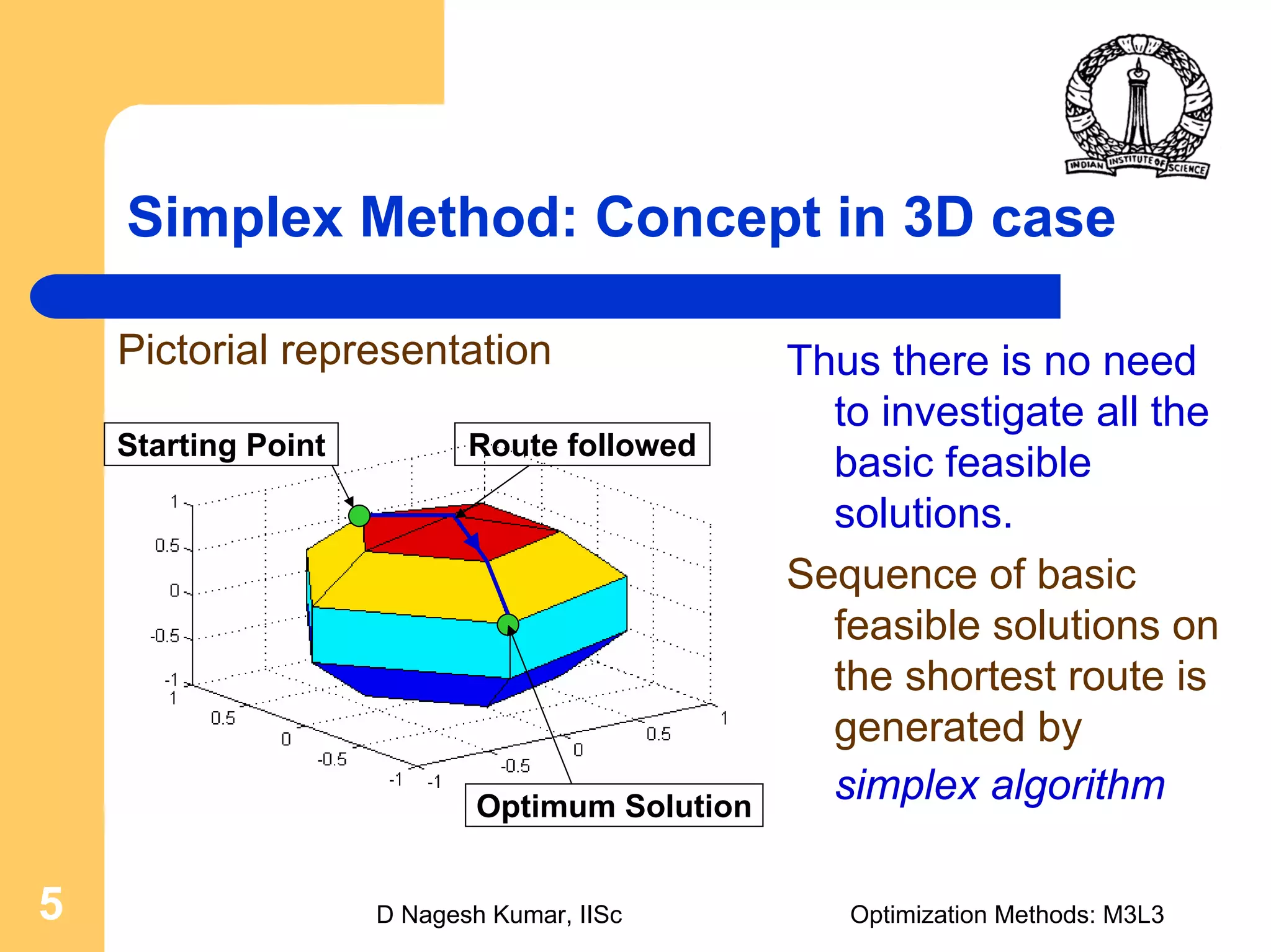
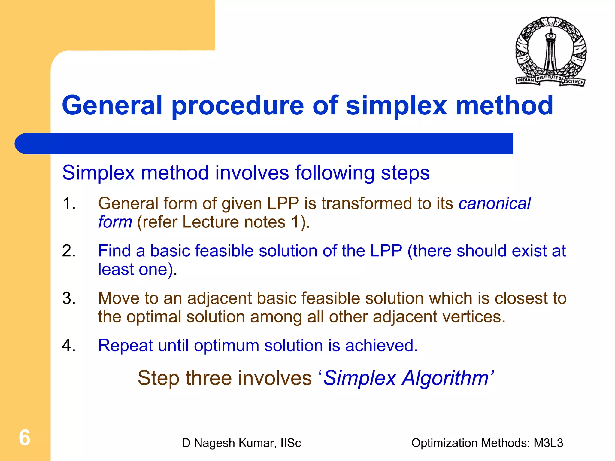
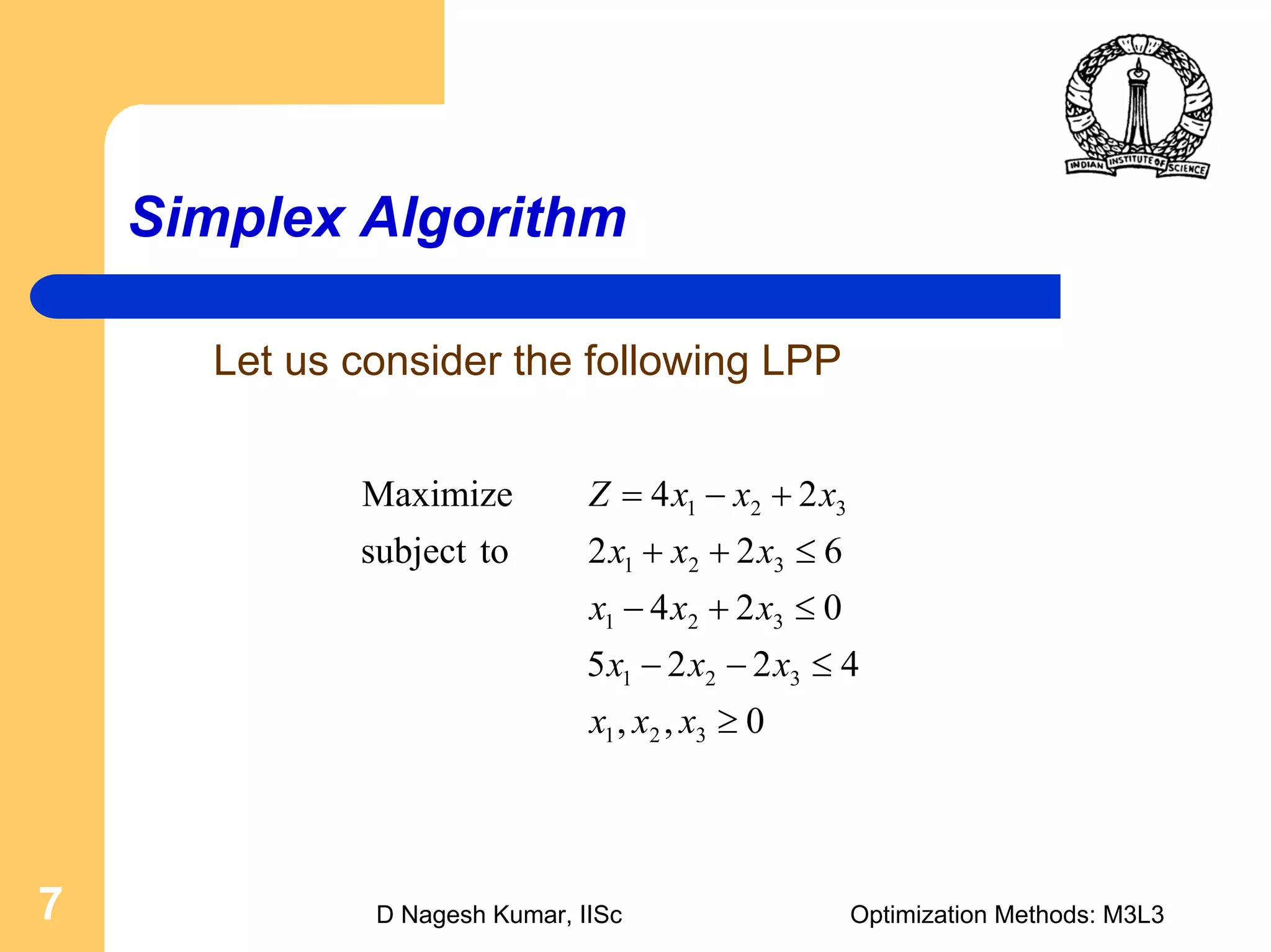

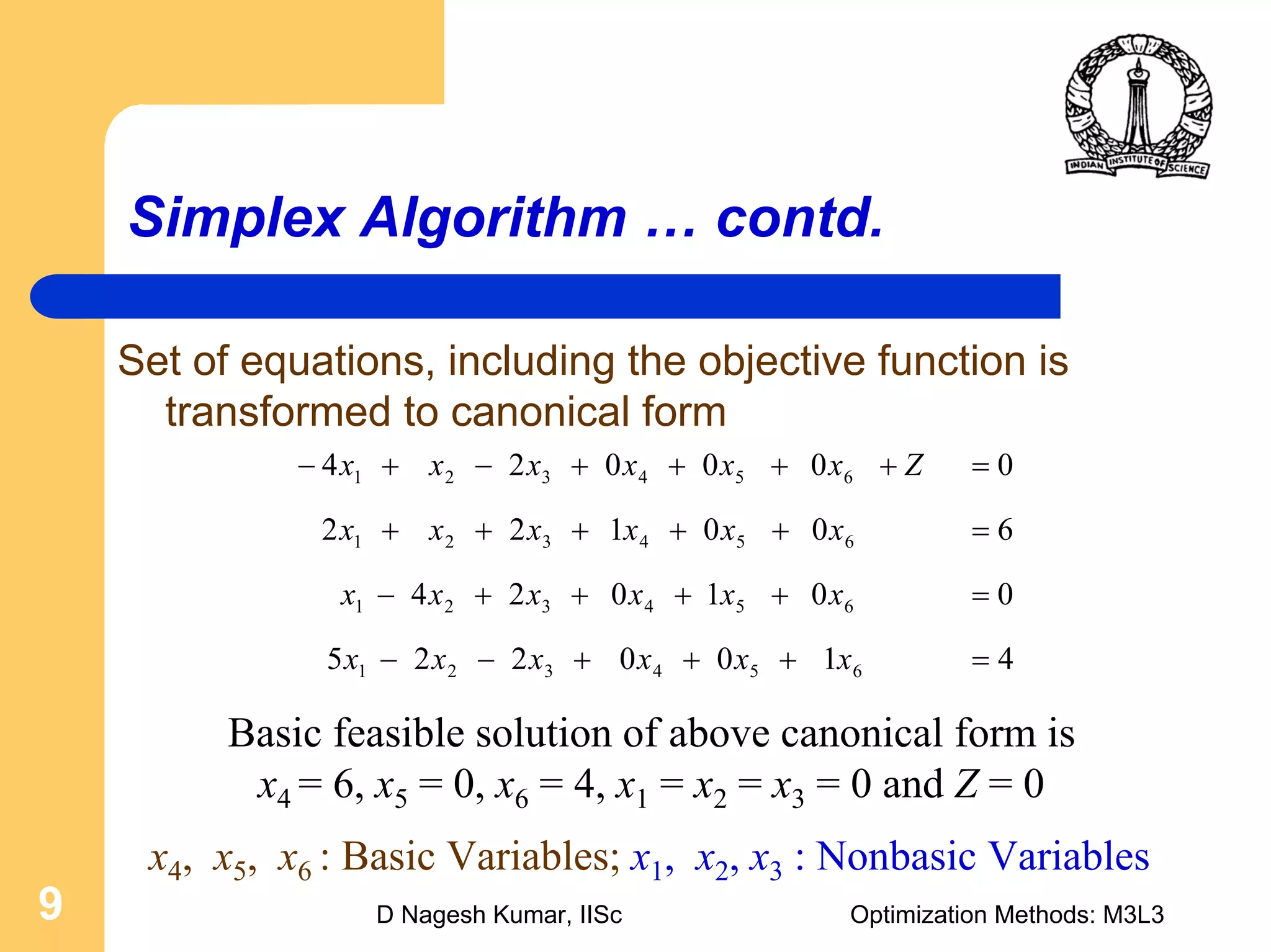


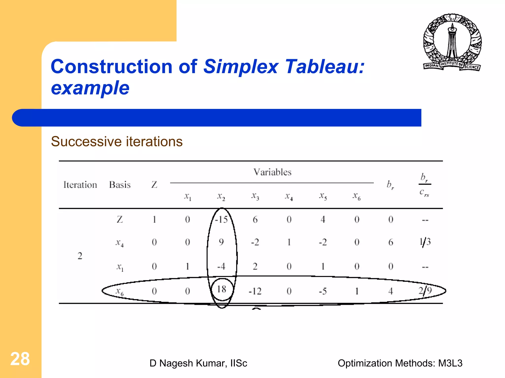
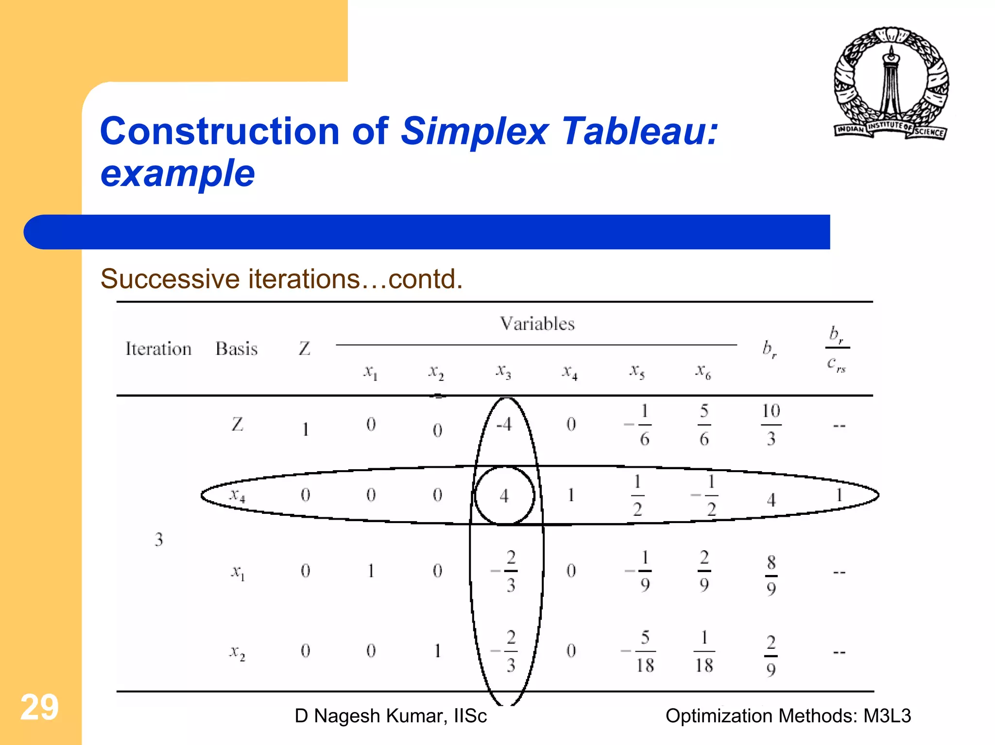
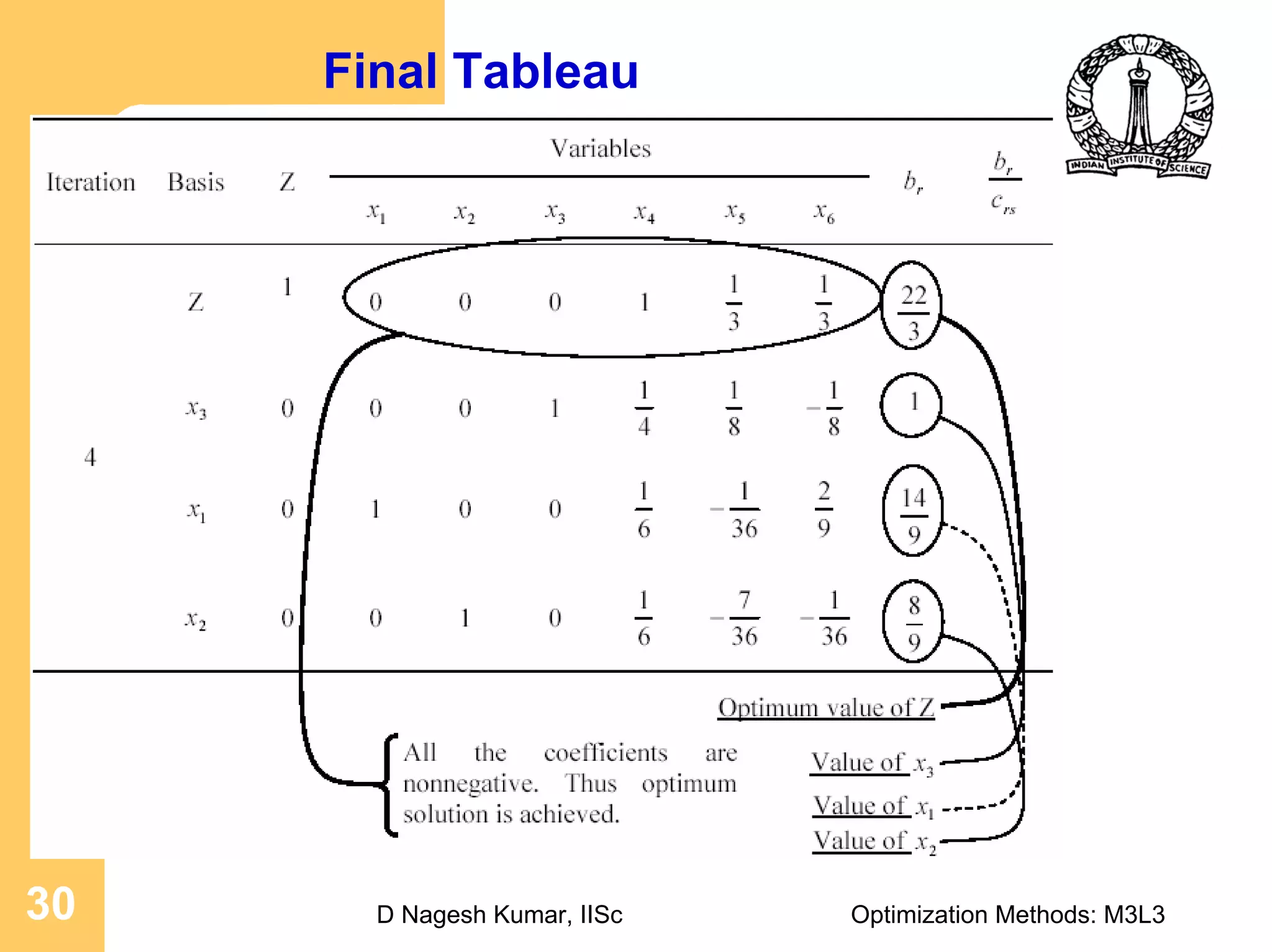
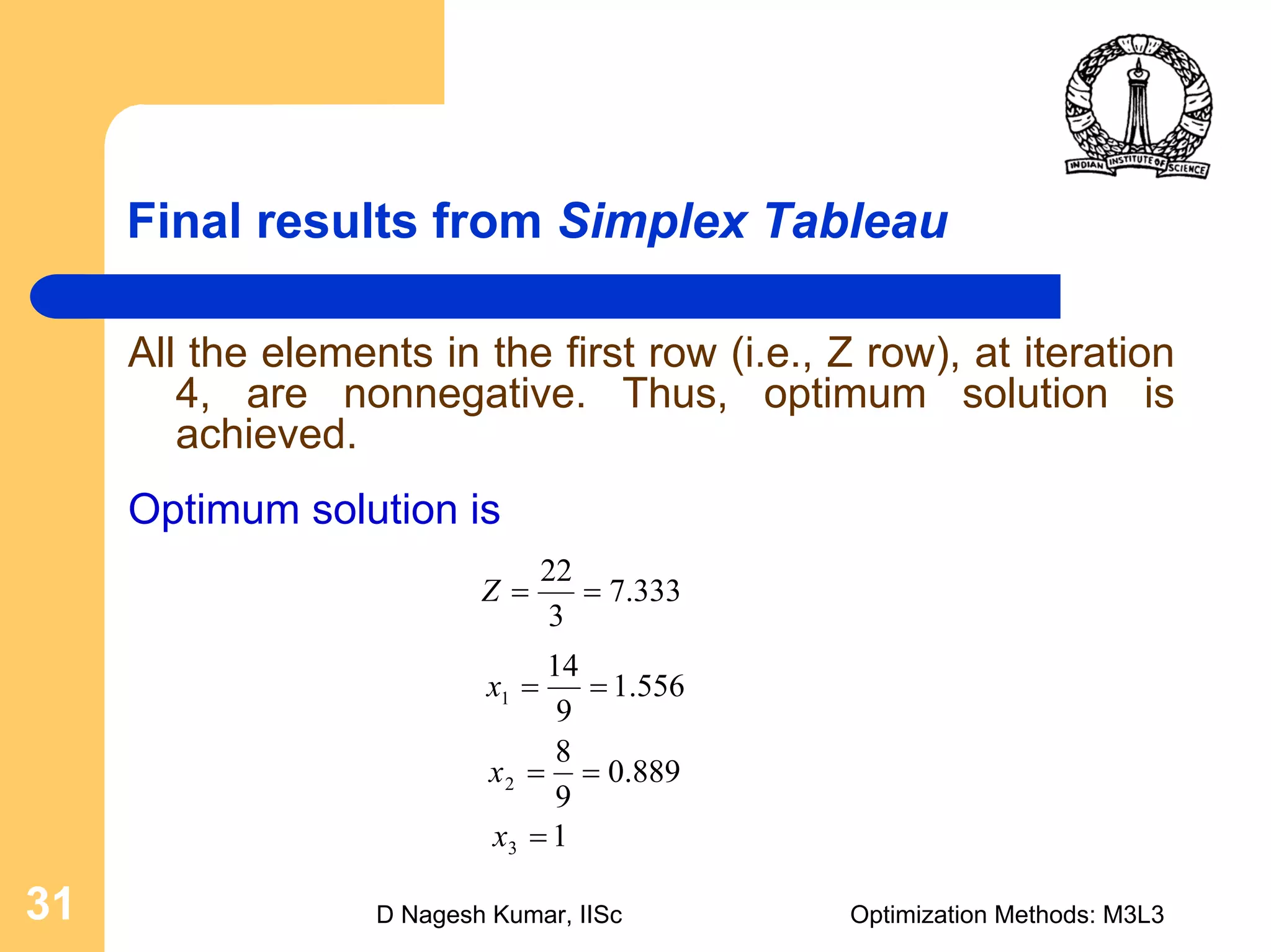
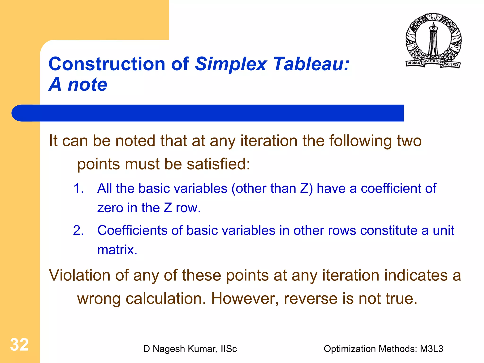

The document discusses the simplex method for solving linear programming problems. It begins by introducing linear programming and the objectives of discussing the simplex method algorithm and demonstrating the construction of simplex tableaus. It then provides motivation for the simplex method by explaining how it can be used to find the optimal solution more efficiently than investigating all possible basic feasible solutions individually. The concept of the simplex method is explained visually in 3D. The general procedure is outlined as transforming the problem to canonical form, finding an initial basic feasible solution, and then moving between adjacent basic feasible solutions until the optimum is found. An example problem is solved step-by-step using the simplex method and presented in a simplex tableau.


![Digital Signal Processing[ECEG-3171]-Ch1_L02](https://cdn.slidesharecdn.com/ss_thumbnails/dspl2-180427094423-thumbnail.jpg?width=640&height=640&fit=bounds)