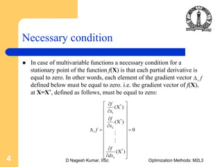
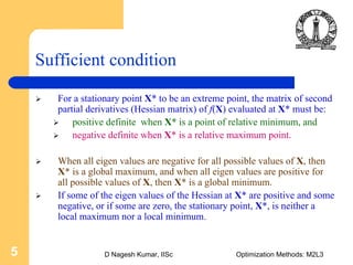
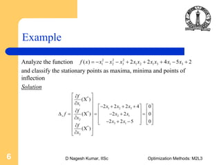
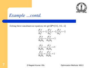
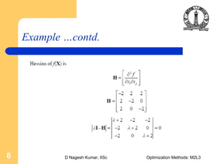
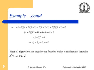
This document discusses unconstrained optimization of functions with multiple variables. It explains that the gradient vector and Hessian matrix are used to analyze these types of functions. The necessary condition for a stationary point is that the gradient vector must be equal to zero. The sufficient condition is that the Hessian matrix must be positive definite for a minimum or negative definite for a maximum. An example function is analyzed to classify its stationary points as maxima, minima or points of inflection. The solutions and working are shown step-by-step for this example.

1. D Nagesh Kumar, IISc Optimization Methods: M2L31
Optimization using Calculus
Optimization of
Functions of Multiple
Variables: Unconstrained
Optimization

2. D Nagesh Kumar, IISc Optimization Methods: M2L32
Objectives
To study functions of multiple variables, which are more difficult to
analyze owing to the difficulty in graphical representation and
tedious calculations involved in mathematical analysis for
unconstrained optimization.
To study the above with the aid of the gradient vector and the
Hessian matrix.
To discuss the implementation of the technique through examples

3. D Nagesh Kumar, IISc Optimization Methods: M2L33
Unconstrained optimization
If a convex function is to be minimized, the stationary point is the
global minimum and analysis is relatively straightforward as
discussed earlier.
A similar situation exists for maximizing a concave variable function.
The necessary and sufficient conditions for the optimization of
unconstrained function of several variables are discussed.

4. D Nagesh Kumar, IISc Optimization Methods: M2L34
Necessary condition
In case of multivariable functions a necessary condition for a
stationary point of the function f(X) is that each partial derivative is
equal to zero. In other words, each element of the gradient vector
defined below must be equal to zero. i.e. the gradient vector of f(X),
at X=X*, defined as follows, must be equal to zero:
x fΔ
*
1
*
2
*
( )
( )
0
( )
x
n
f
x
f
x
f
f
dx
∂⎡ ⎤
Χ⎢ ⎥∂
⎢ ⎥
∂⎢ ⎥
Χ⎢ ⎥∂
⎢ ⎥Δ = =
⎢ ⎥
⎢ ⎥
⎢ ⎥
⎢ ⎥∂
Χ⎢ ⎥
∂⎣ ⎦
M
M

5. D Nagesh Kumar, IISc Optimization Methods: M2L35
Sufficient condition
For a stationary point X* to be an extreme point, the matrix of second
partial derivatives (Hessian matrix) of f(X) evaluated at X* must be:
positive definite when X* is a point of relative minimum, and
negative definite when X* is a relative maximum point.
When all eigen values are negative for all possible values of X, then
X* is a global maximum, and when all eigen values are positive for
all possible values of X, then X* is a global minimum.
If some of the eigen values of the Hessian at X* are positive and some
negative, or if some are zero, the stationary point, X*, is neither a
local maximum nor a local minimum.

6. D Nagesh Kumar, IISc Optimization Methods: M2L36
Example
Analyze the function
and classify the stationary points as maxima, minima and points of
inflection
Solution
2 2 2
1 2 3 1 2 1 3 1 3( ) 2 2 4 5 2f x x x x x x x x x x= − − − + + + − +
*
1
1 2 3
*
2 1
2
3 1
*
3
( )
2 2 2 4 0
( ) 2 2 0
2 2 5 0
( )
x
f
x
x x x
f
f x x
x
x x
f
x
⎡ ⎤∂
Χ⎢ ⎥
∂⎢ ⎥ − + + +⎡ ⎤ ⎡ ⎤
⎢ ⎥∂ ⎢ ⎥ ⎢ ⎥Δ = Χ = − + =⎢ ⎥ ⎢ ⎥ ⎢ ⎥∂⎢ ⎥ ⎢ ⎥ ⎢ ⎥− + −⎣ ⎦ ⎣ ⎦⎢ ⎥∂
Χ⎢ ⎥
∂⎣ ⎦

7. D Nagesh Kumar, IISc Optimization Methods: M2L37
Example …contd.

8. D Nagesh Kumar, IISc Optimization Methods: M2L38
Example …contd.

9. D Nagesh Kumar, IISc Optimization Methods: M2L39
Example …contd.

10. D Nagesh Kumar, IISc Optimization Methods: M2L310
Thank you