Downloaded 31 times

The document summarizes the simplex method for solving linear programming problems involving maximization. It involves 12 steps: 1) Formulating the LPP, 2) Introducing slack, surplus and artificial variables, 3) Formulating the initial basic solution, 4) Constructing the initial simplex table, 5) Checking for positive elements in the Cj-Zj row, 6) Identifying the incoming basic variable, 7) Choosing the incoming basic variable if multiple positives exist, 8) Identifying the outgoing basic variable, 9) Constructing the next simplex table using row operations, 10) Completing the new simplex table, 11) Repeating steps 5-10, and 12) Terminating when the
Introduction to the Simplex Method focused on maximization problems.
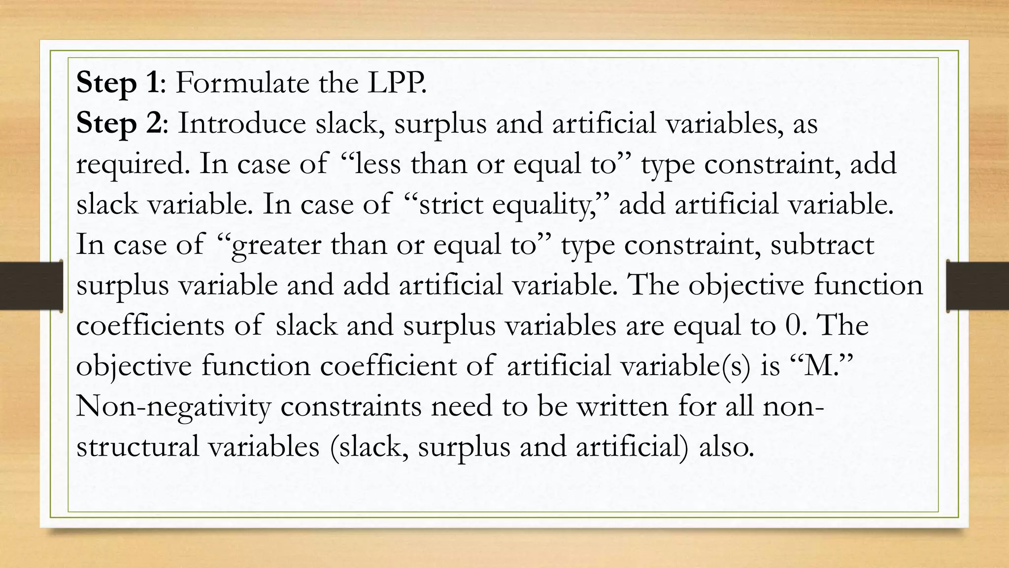
Steps to formulate Linear Programming Problems (LPP), introducing slack, surplus, and artificial variables.
Formulating the initial basic solution ensuring non-negativity and constraints alignment.
Constructing the simplex table including basic variables, coefficients, and solution values.
Continued construction of the simplex table, detailing variable coefficients.
Calculating Zj and Cj-Zj rows for the initial simplex table.
Examine Cj-Zj row for positive elements; indicates whether maximum objective value is found.
Identifying the incoming basic variable based on Cj-Zj values in the simplex table.
Determining the outgoing basic variable using ratios from the optimum column.
Constructing the next simplex table with updated basic variable replacements.
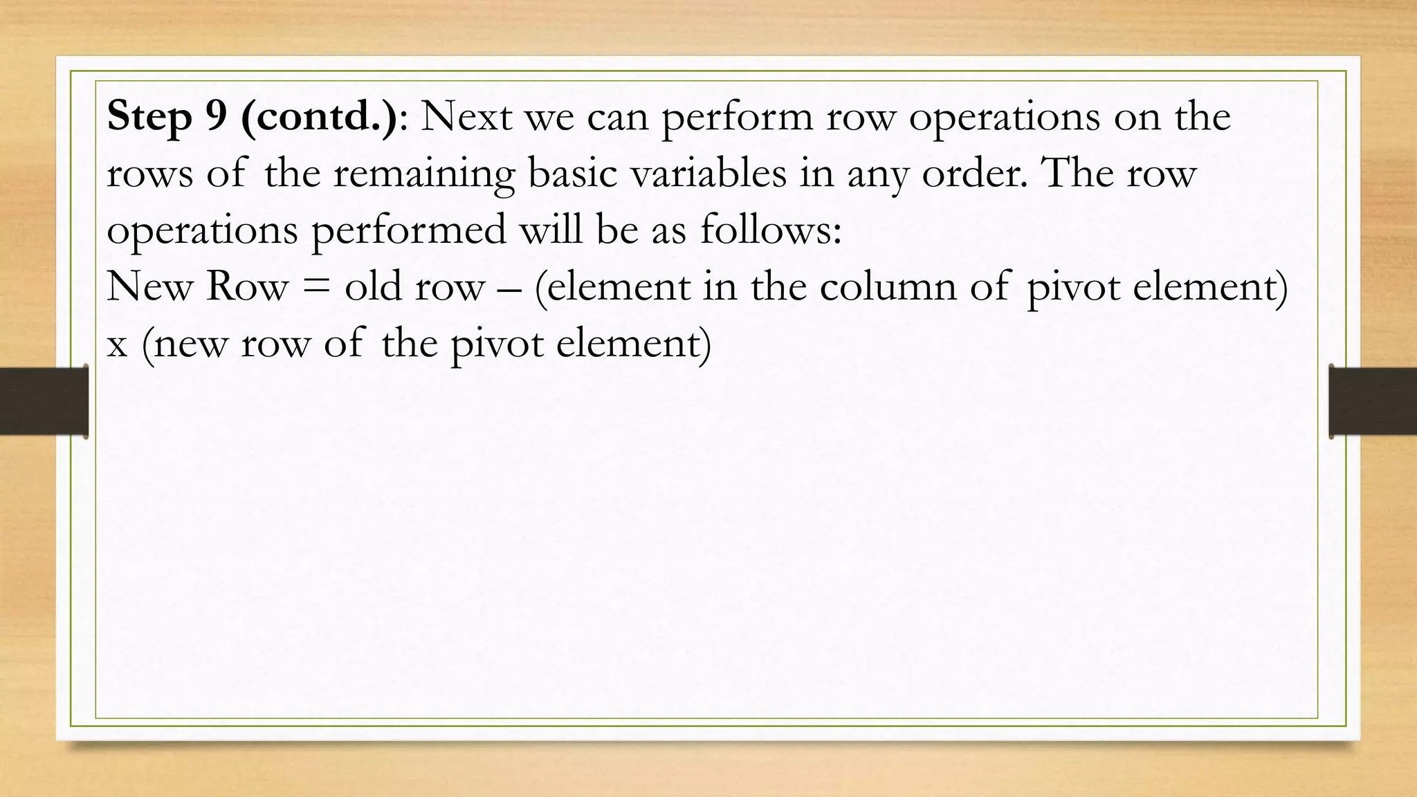
Row operations on remaining basic variables for the updated simplex table.
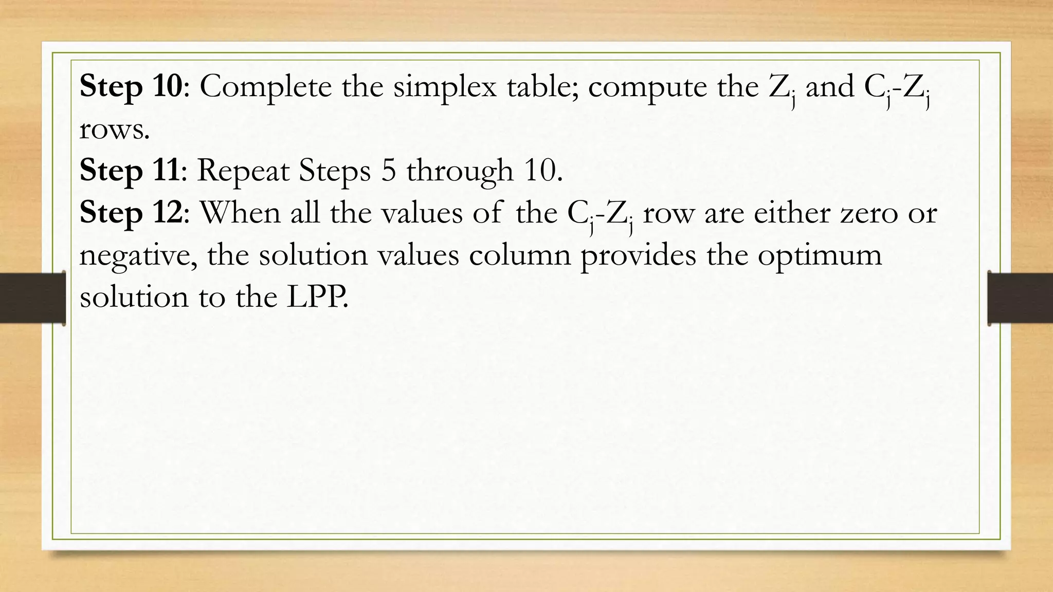
Completing the simplex table and obtaining the optimal solution when Cj-Zj is non-positive.