Downloaded 93 times


The document provides an overview of the simplex algorithm, which is used to solve linear programming problems. It defines key terms like standard form, slack variables, basic and non-basic variables, and pivoting. The simplex algorithm involves writing the problem in standard form, selecting a pivot column and row, and performing row operations to find an optimal solution. An example problem is worked through in multiple iterations to demonstrate how the algorithm progresses from an initial tableau to the optimal solution. Potential issues like cycling are also discussed, along with software tools to implement the simplex method.
Muhammad Kashif Nawaz, MS(CS) Batch # 3, Email: Kashif.rpb@gmail.com.
Overview of contents: Introduction, Key Terminologies, Simplex Algorithm, Software Simulation, Variations, References.
Linear programming optimizes outcomes using inequalities. Important for optimization techniques.
Graphical methods are inadequate for complex LP problems; hence the Simplex Algorithm is required.
Introduced by George B. Dantzig in 1947; recognized as a top algorithm for solving Linear Programming Problems.
Standard Form, Slack Variable, Basic & Nonbasic Variables, Simple Tableau, Pivoting.
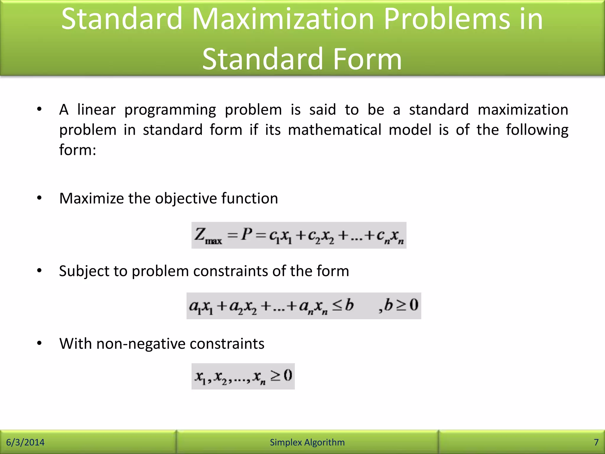
Standard maximization form: maximize objective function with non-negative constraints.
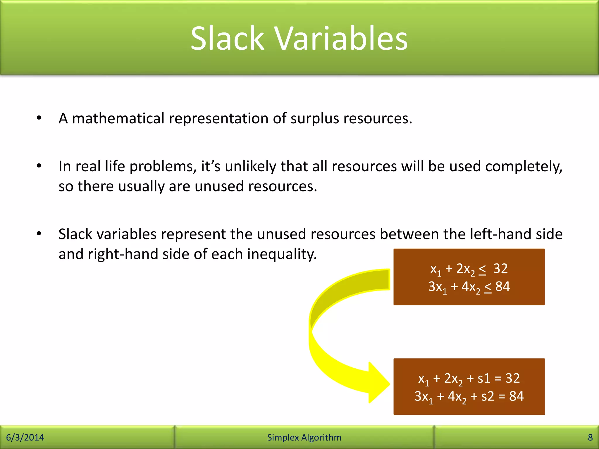
Represents surplus in resources; helps identify unused resources in LP inequalities.
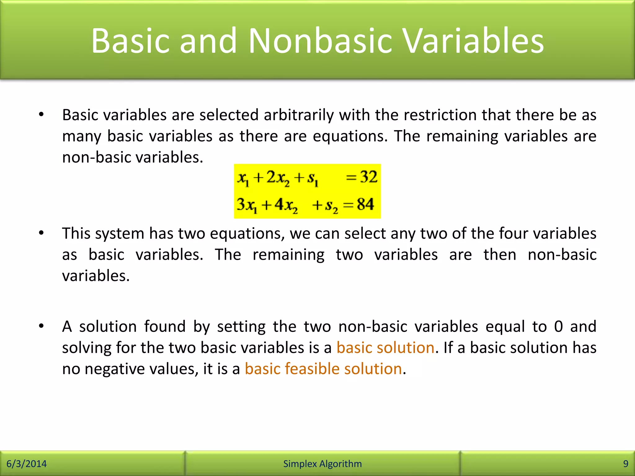
Definition of basic and non-basic variables; importance in forming basic feasible solutions.
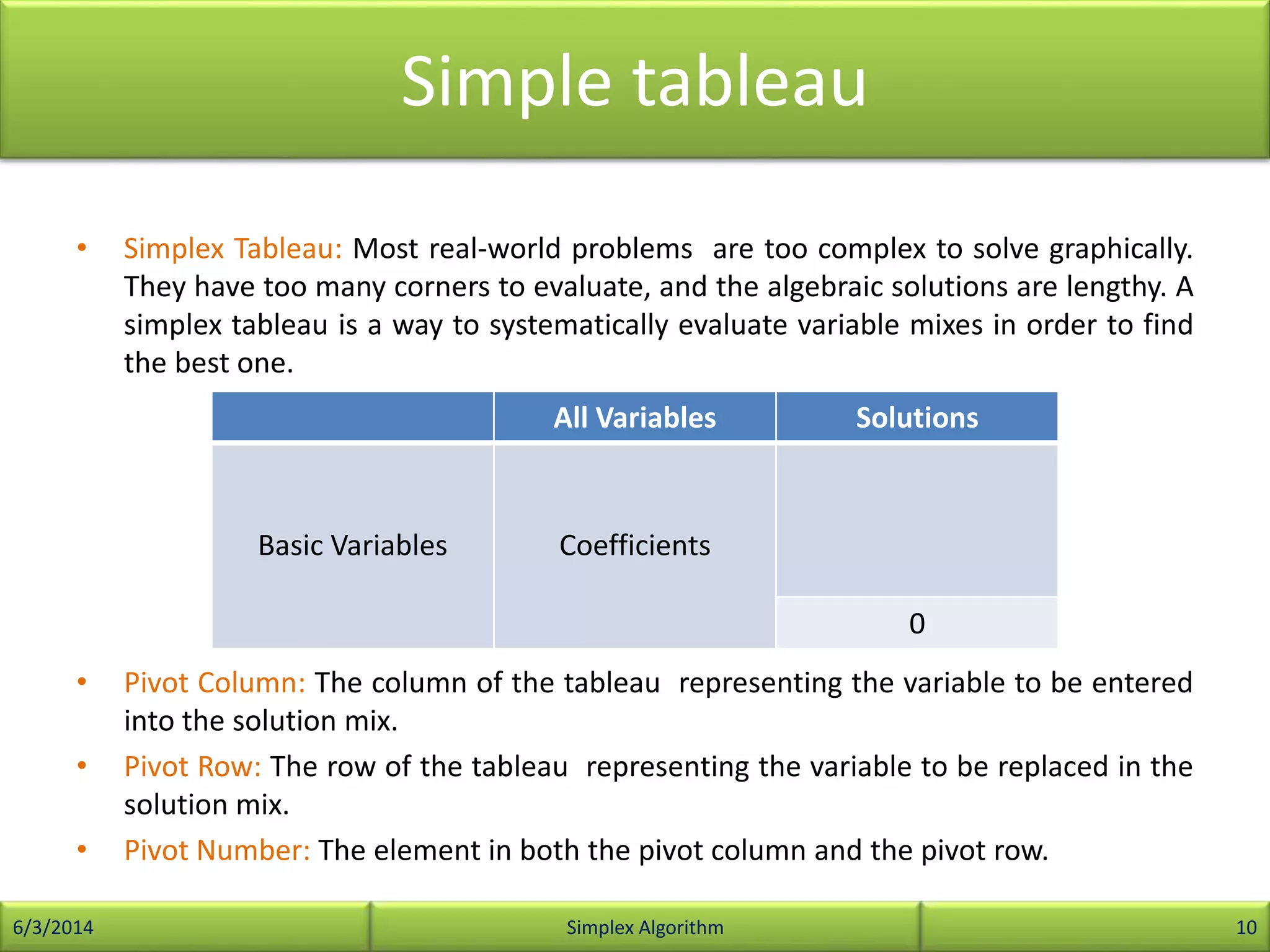
Systematic evaluation technique for solving LP problems using Simplex Tableau, including definitions.
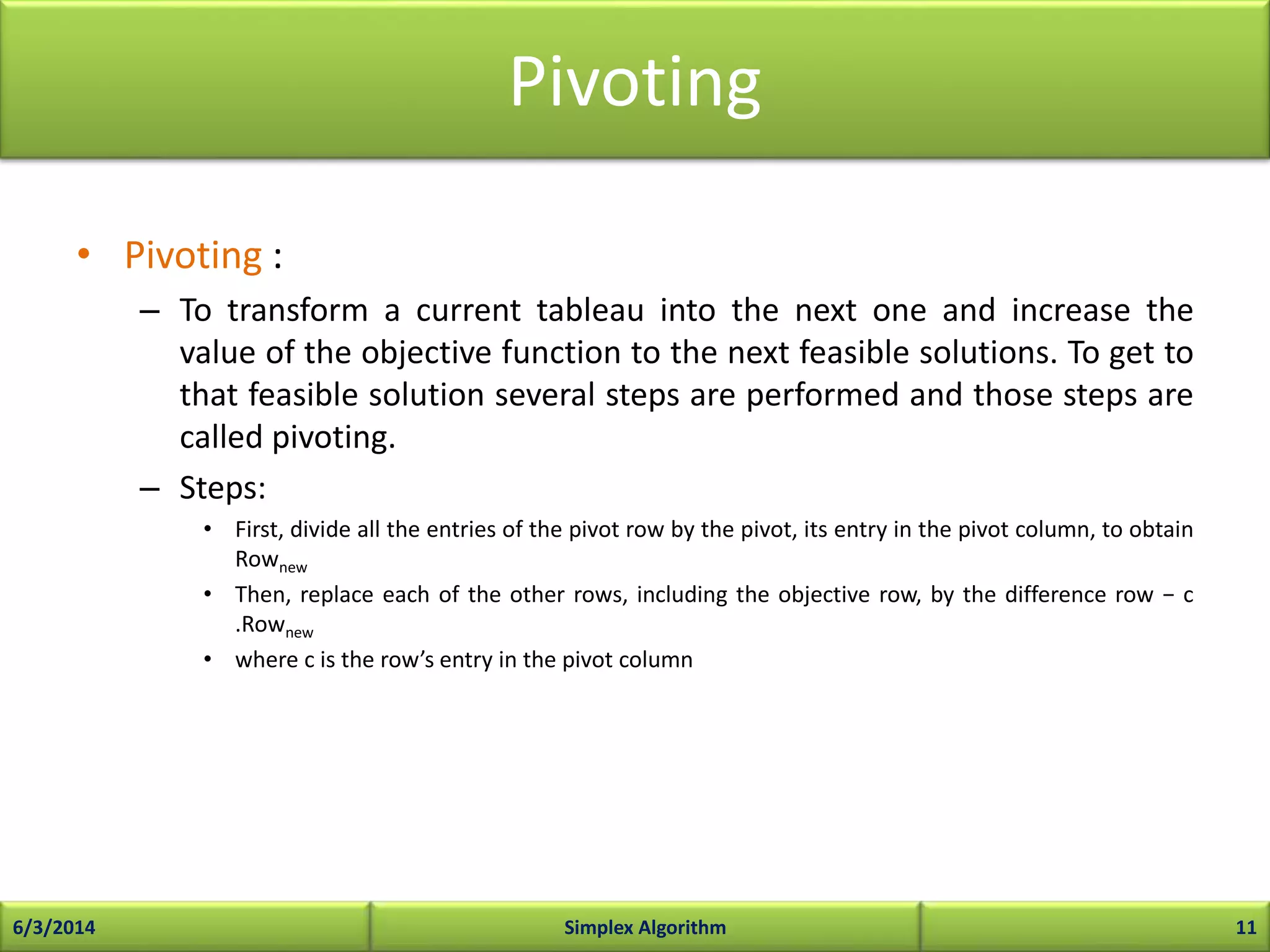
Stepwise transformation of tableau, essential for improving objective function value.
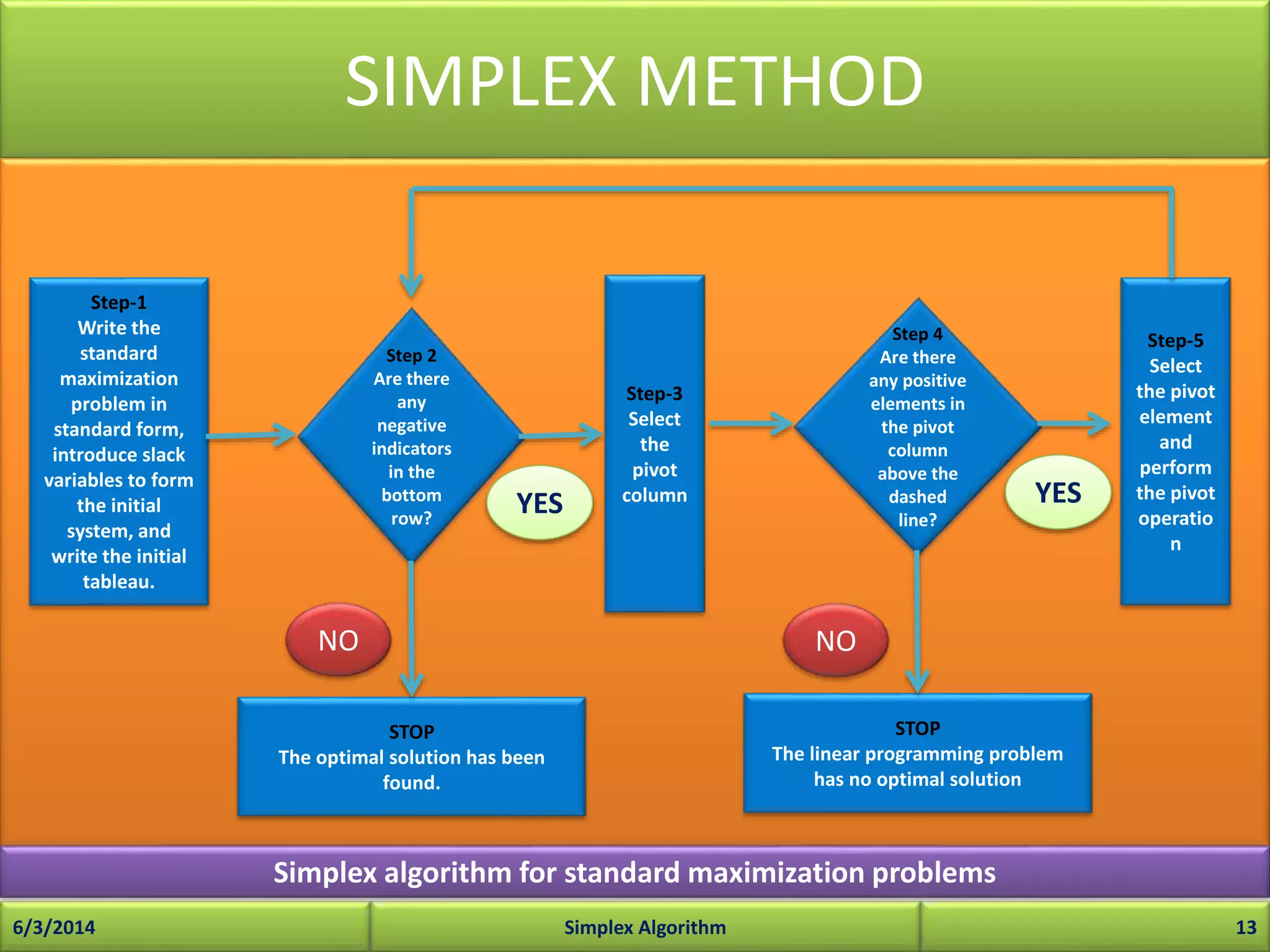
Steps in applying Simplex Algorithm, including critical considerations and calculations.
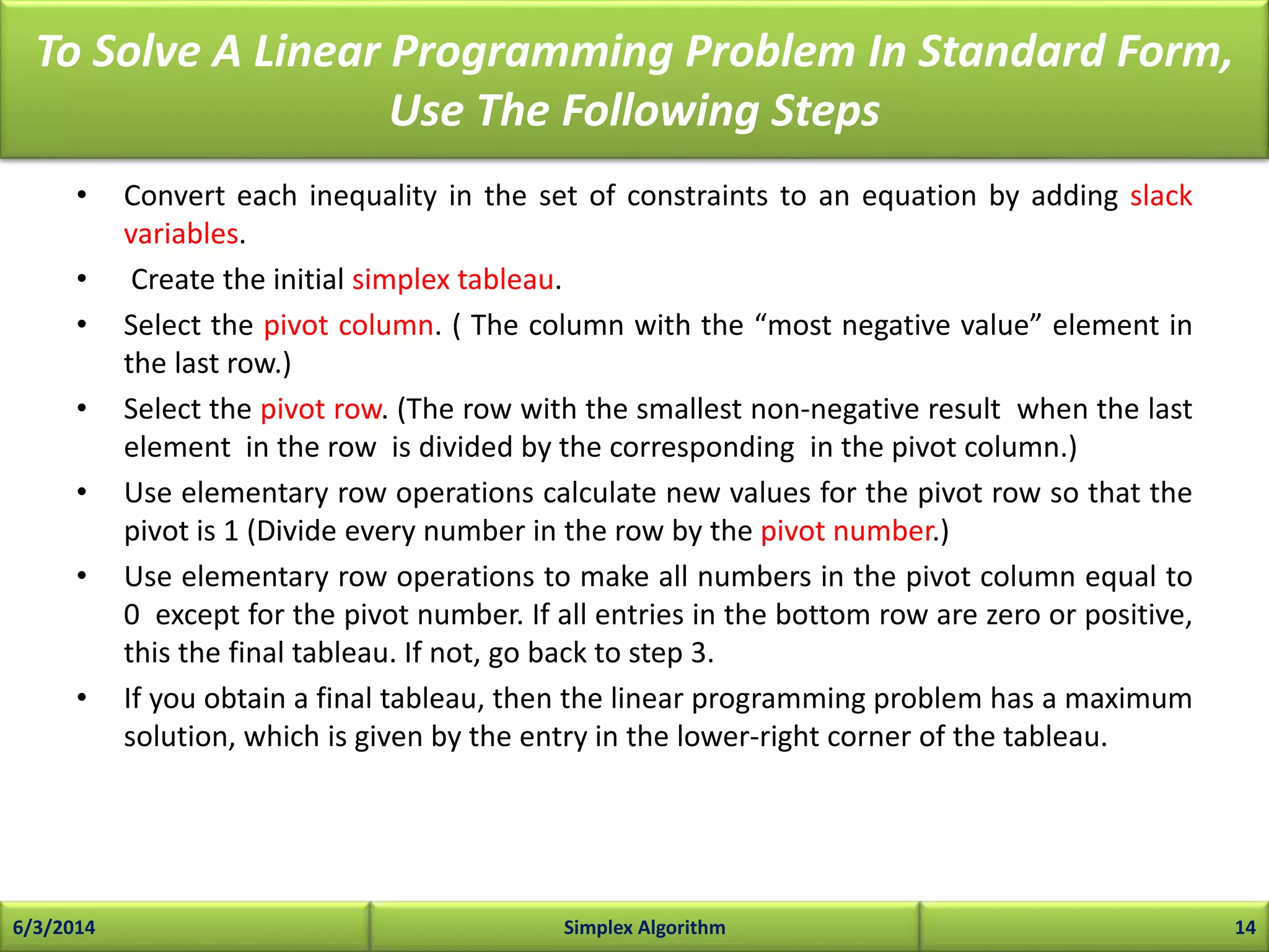
Detailed steps involved in executing the Simplex method for maximization problems.
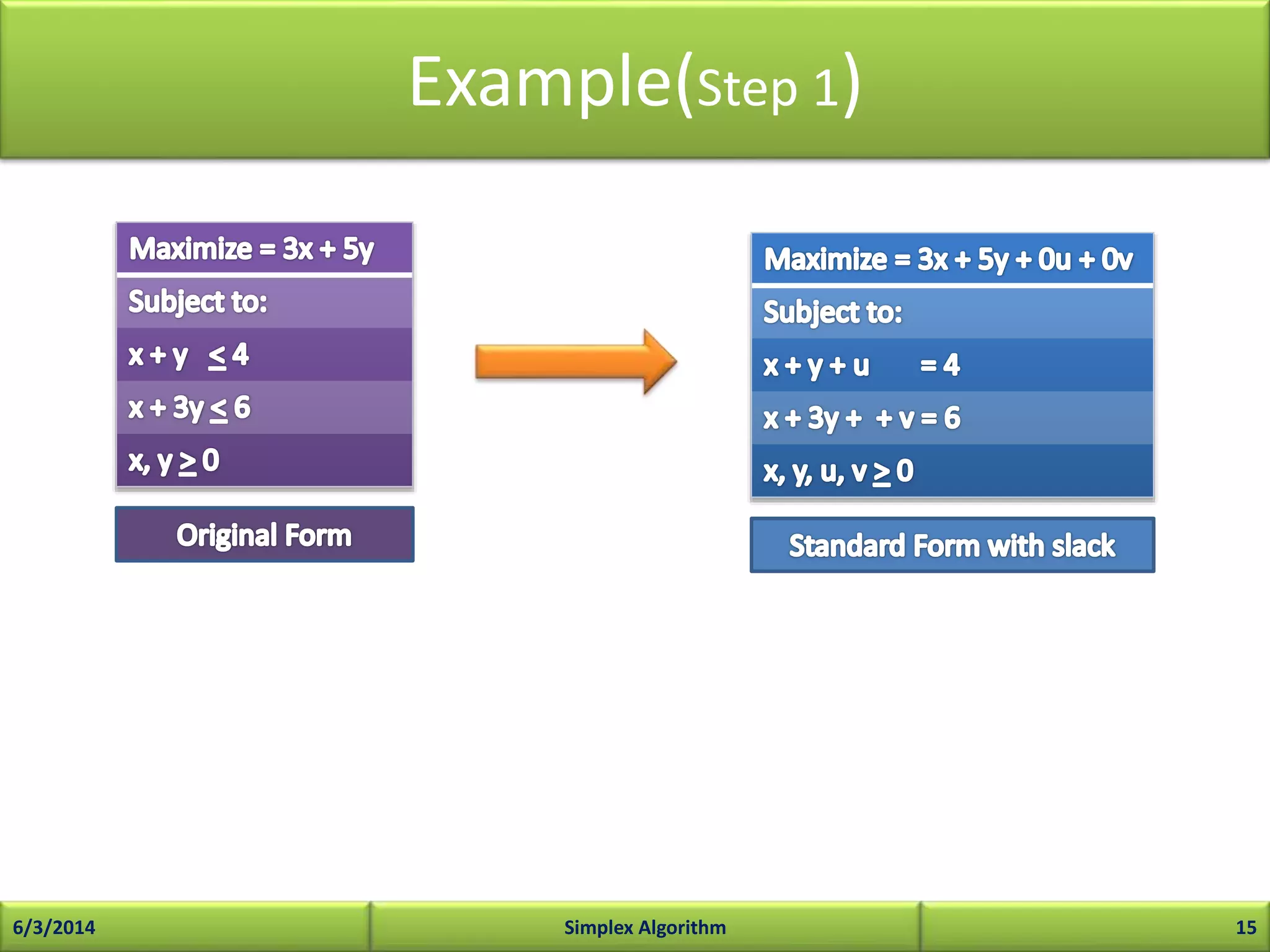
Instructions for converting inequalities to equations using slack variables and tableau creation.
Initial setup for simplex algorithm example.
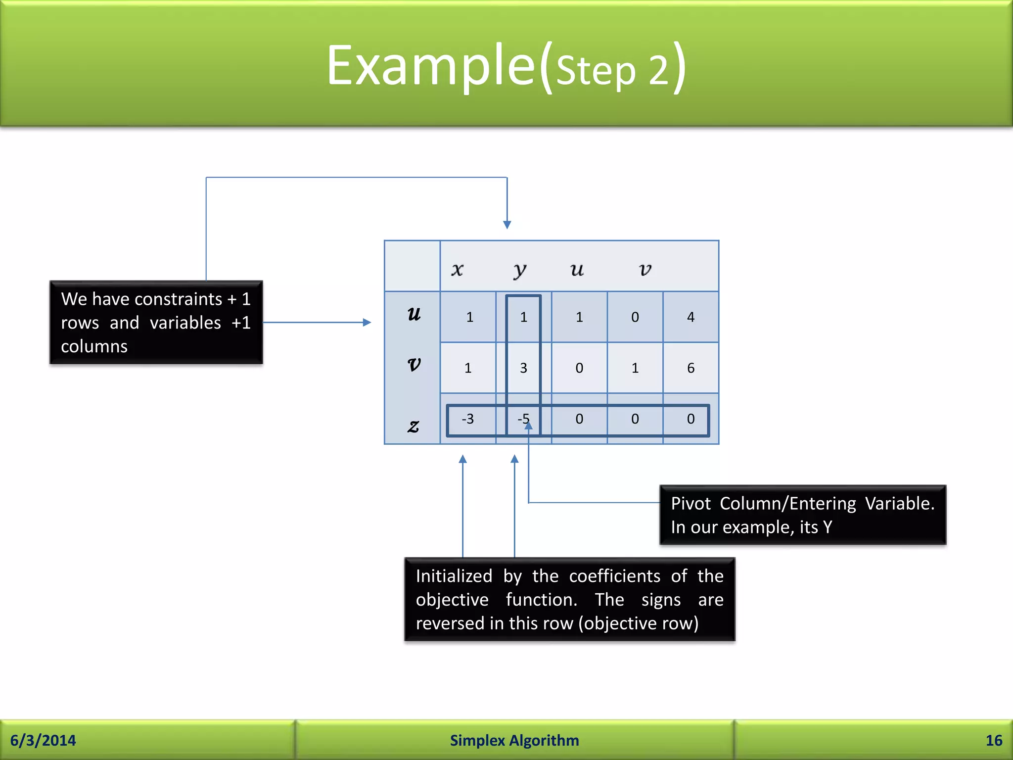
Setting up the tableau with initial coefficients for objective function and constraints.
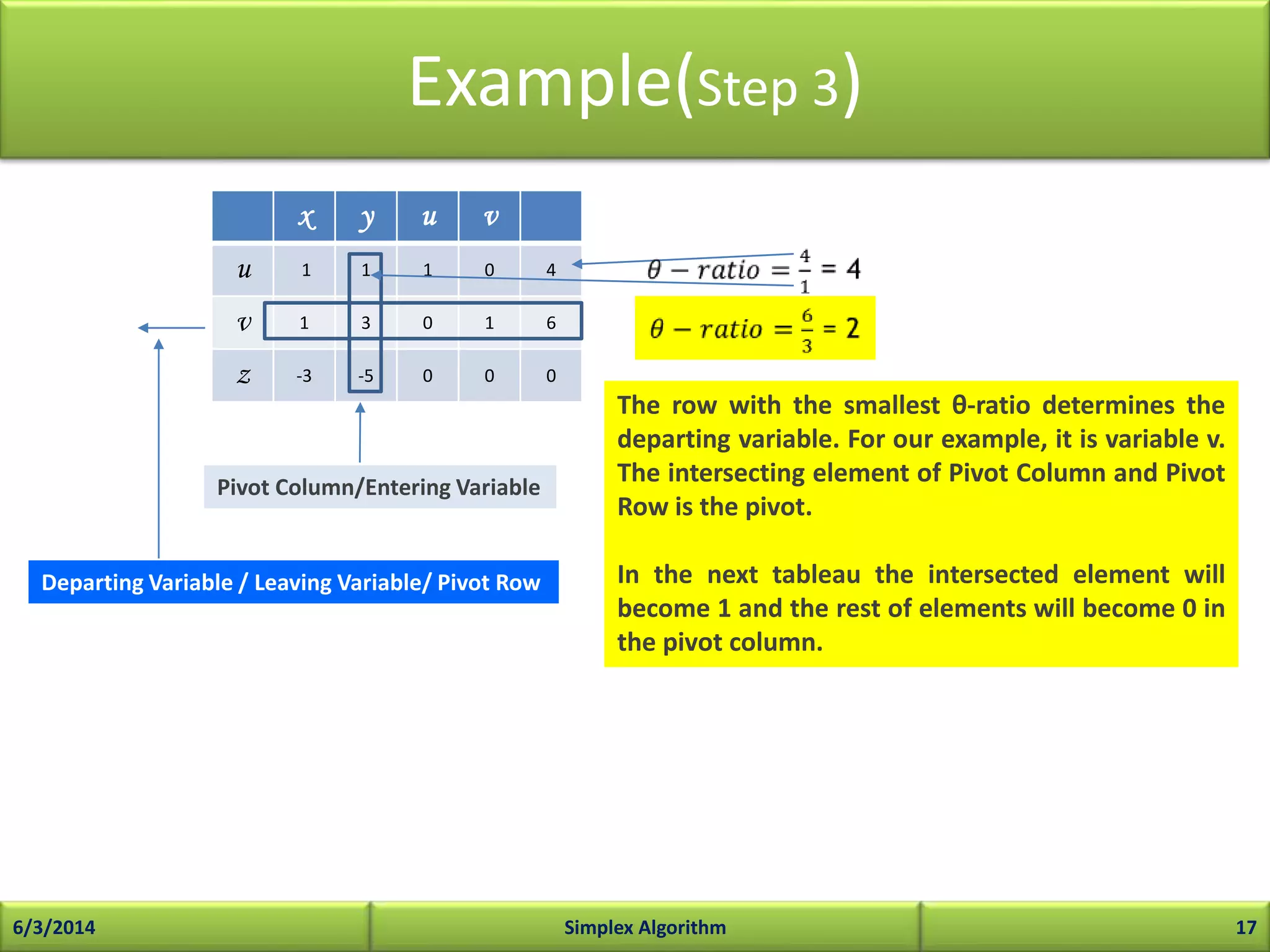
Determining entering variable and pivot row in tableau.
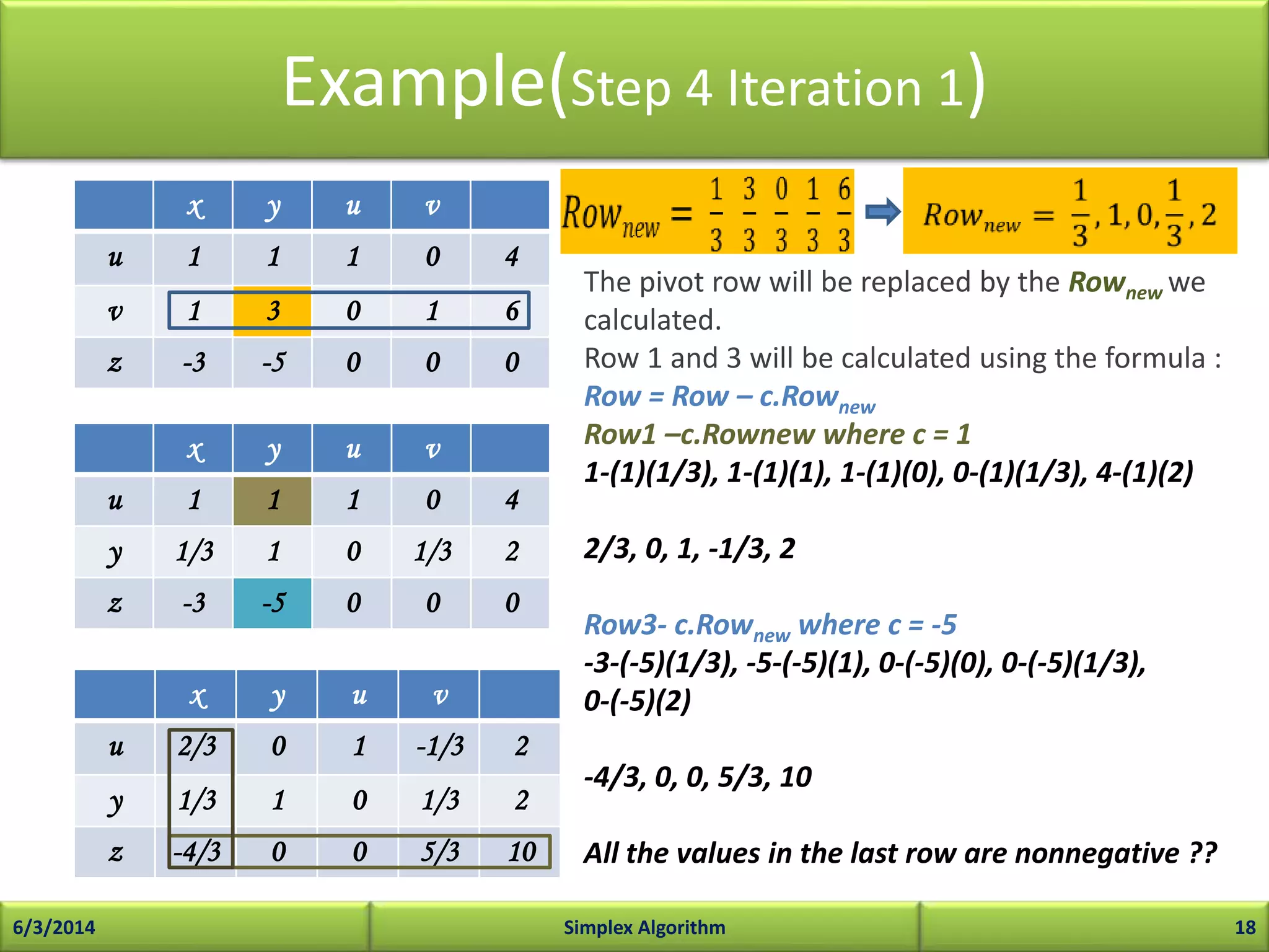
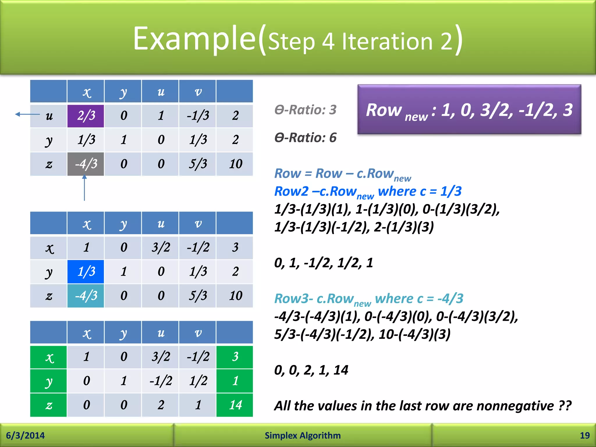
First iterative step adjustments in tableau; calculation of new values.
Continuation of tableau adjustments leading to potential optimal solution.
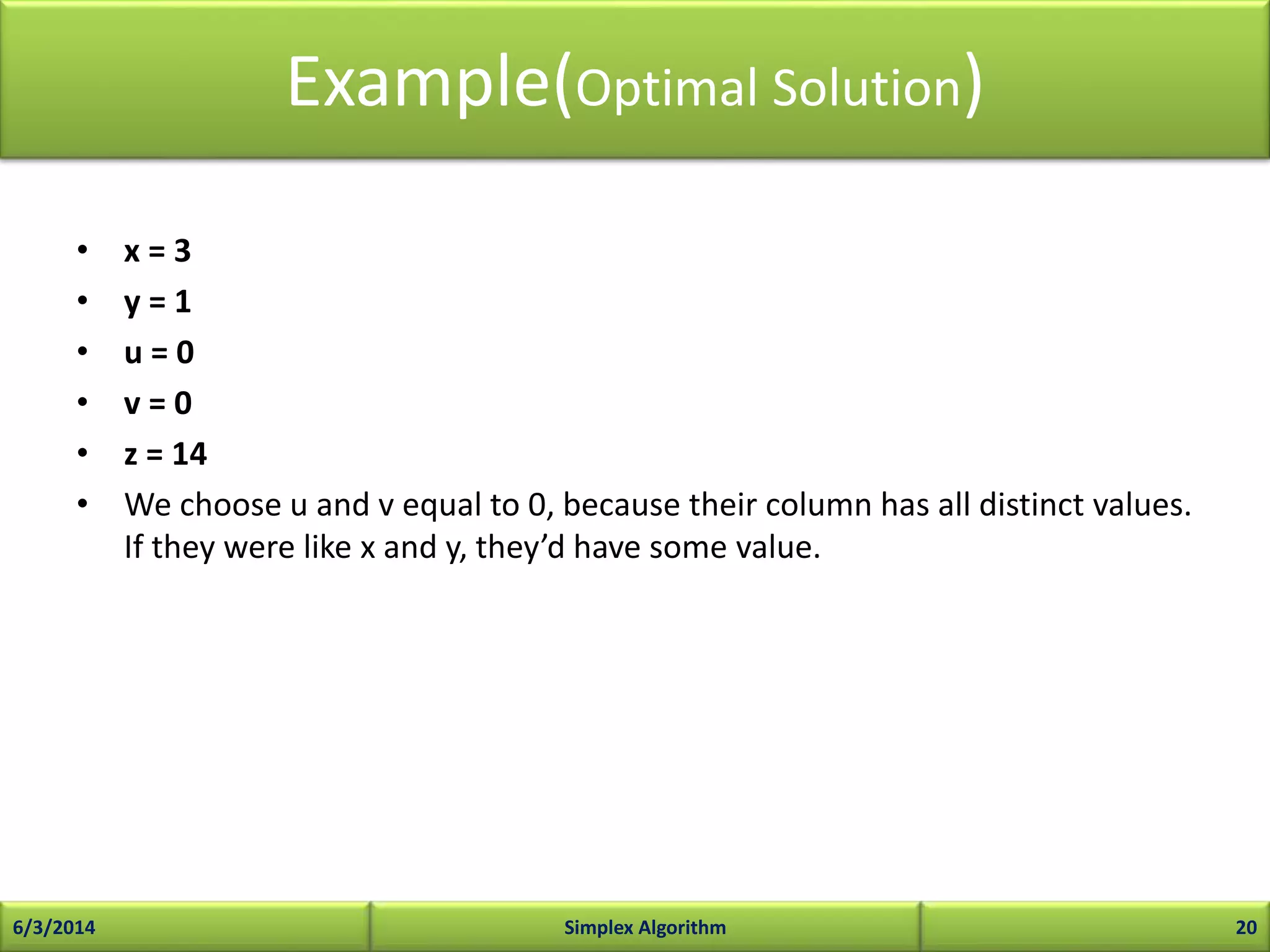
Final results indicate optimal values for decision variables in the LP problem.
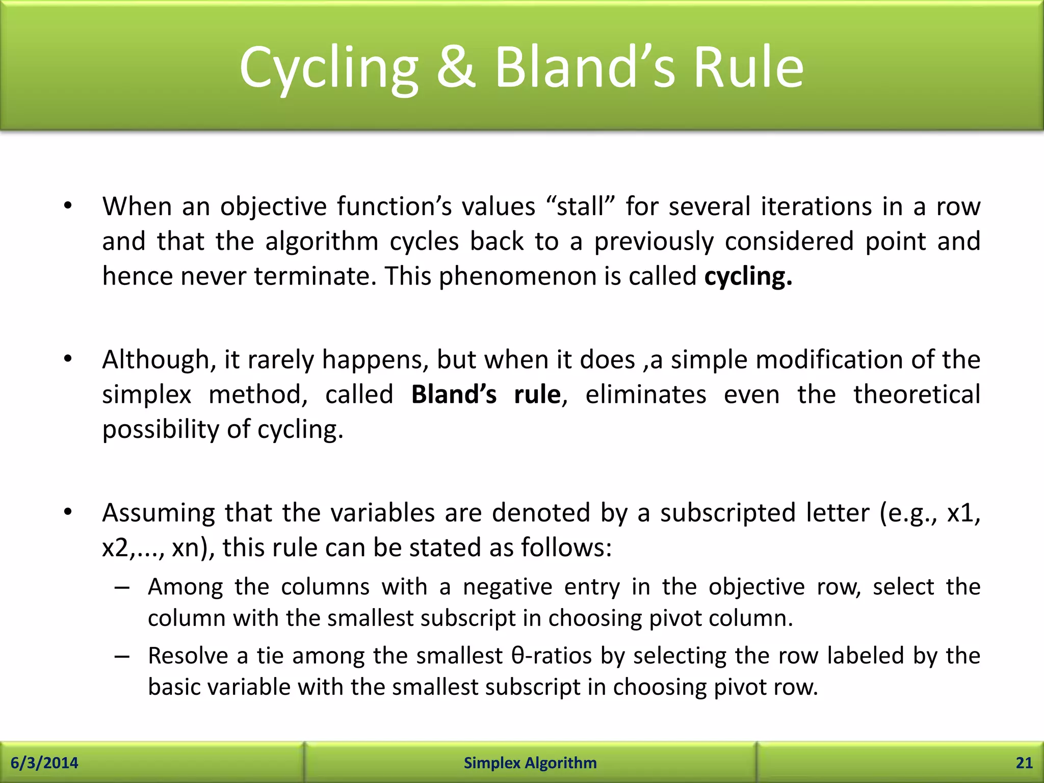
Discussion on cycling issues in simplex process and solution using Bland’s rule.
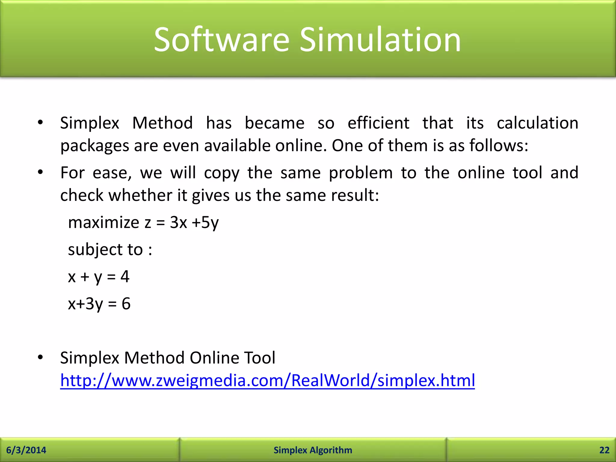
Presentation of online tools available for performing simplex calculations.
Efficiency characteristics and typical iteration ranges of simplex algorithm in practice.
Brief overview of other methods: Ellipsoid Method and Karmarker's Method.
Cited sources include key textbooks and online material relevant to the presentation.