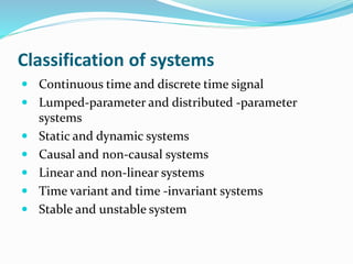
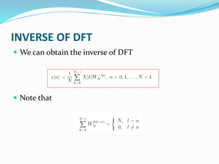
This document summarizes key concepts in digital signal processing systems. It defines a system as a combination of elements that processes an input signal to produce an output signal. Systems are classified as continuous or discrete time, lumped or distributed parameter, static or dynamic, causal or non-causal, linear or non-linear, time variant or invariant, and stable or unstable. Convolution and the discrete Fourier transform (DFT) are also introduced as important tools in digital signal processing. The DFT transforms a signal from the time domain to the frequency domain.

1. Digital Signal Processing
.
Mrs.R.Chitra, Assistant Professor(SS),
Department of ECE,
Faculty of Engineering,
Avinashilingam Institute for Home Science
and Higher Education for Women,
Coimbatore

2. SYSTEM
DEFINITION:
 Combination of set of elements.
 It will process or manipulate over input signal to
produce output signal

3. Classification of systems
 Continuous time and discrete time signal
 Lumped-parameter and distributed -parameter
systems
 Static and dynamic systems
 Causal and non-causal systems
 Linear and non-linear systems
 Time variant and time -invariant systems
 Stable and unstable system

4. Continuous time system
A Continuous time system is one which operates on a
continuous time input signal and produces a continuous
time output signal.
y(t)= Tx(t)

5. Discrete time system
A discrete time system is the one which operates on a
discrete- time input signal and produces a discrete -time
output signal.
y(n)=T(X(n)

6. Lumped and distributed parameter
 In lumped parameter system each component is
lumped at one point in space.
 In distributed parameter systems the signals are
functions of space as well as time.

7. Static and dynamic system
 A system is called static or memory less if its output at
any instant depends on the input at that instant.
 A system output is depends up on the past and future
values of input.

8. Causal and non causal system
 A causal system is one for which the output at any time
t depends on the present and past inputs.
 A non-causal system output depends on the future
values of inputs.

9. Linear and non linear system
A System is said to be linear if it follows super position
principle is called as linear other wise non-linear.
T[ax1(t)+bx2(t)]=aT[x1(t)]+bT[x2(t)]
Similarly for a discrete-time linear system,
T[ax1(n)+bx2(n)]=aT[x1(n)]+bT[x2(n)]

10. Stable and unstable system
 If the system has to be stable if and only if every
bounded input produces bounded output.
 If system has to be unstable if bounded input produces
unbounded output

11. Time variant and invariant system
 Time variant system have same input and output,
y(n,k)=y(n-k).
 Time invariant system has no same input and output.

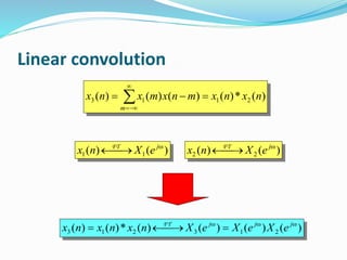
12. CONVOLUTION
 Convolution is the process by which an input interacts
 with an LTI system to produce an output
 Convolution between of an input signal x[n] with a
 system having impulse response h[n] is given as,
 where * denotes the convolution
 x [ n ] * h [ n ] = x [ k ] h [ n - k ]

13. EXAMPLE
 Convolution
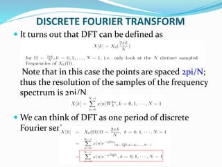
 We can write x[n] (a periodic function) as an infinite
sum of the function xo[n] (a non-periodic function)
shifted N units at a time

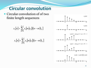
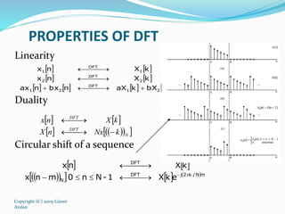
14. Properties of convolution
Commutative…
 x1[n]* x2[n] = x2[n]* x1[n]
Associative…
 {x1[n]* x2 [n]}* x3[n] = x1[n]*{x2 [n]* x3[n]}
Distributive…
 {x1[n] *x2[n]}* x3[n] = x1[n]x3[n] * x2[n]x3[n]

15. Linear convolution
)(*)()()()( 2113 nxnxmnxmxnx
m
 


)()( 11

 j
eXnx FT
)()( 22

 j
eXnx FT
)()()()(*)()( 213213

 jjj
eXeXeXnxnxnx FT

16. Circular convolution
 Circular convolution of of two
finite length sequences
16
       



1
0
213
N
m
Nmnxmxnx
       



1
0
123
N
m
Nmnxmxnx

17. Circular convolution
)()())(()()( 21
1
0
13 nxnxmnxmxnx
N
m
N  


)()( 11 kXnx  DFT
)()( 22 kXnx  DFT
)()()()()()( 213213 kXkXkXnxnxnx   DFT
both of length N

18. EXAMPLE
)()( 01 nnnx 
)(2 nx
)(*)( 21 nxnx
0
0 N
0 n0 N
)()( 21 nxnx 
n0=2, N=7
0

19. DISCRETE FOURIER TRANSFORM
 It turns out that DFT can be defined as
Note that in this case the points are spaced 2pi/N;
thus the resolution of the samples of the frequency
spectrum is 2pi/N.
 We can think of DFT as one period of discrete
Fourier series

20. EXAMPLE OF DFT
 Find X[k]
 We know k=1,.., 7; N=8

21. PROPERTIES OF DFT
Linearity
Duality
Circular shift of a sequence
Copyright (C) 2005 Güner
Arslan
   
   
       kbXkaXnbxnax
kXnx
kXnx
21
DFT
21
2
DFT
2
1
DFT
1
 
 
 
   
       mN/k2jDFT
N
DFT
ekX1-Nn0mnx
kXnx

 
 
   
     N
DFT
DFT
kNxnX
kXnx
 
 

22. INVERSE OF DFT
 We can obtain the inverse of DFT
 Note that

23. EXAMPLE OF IDFT
Remember: