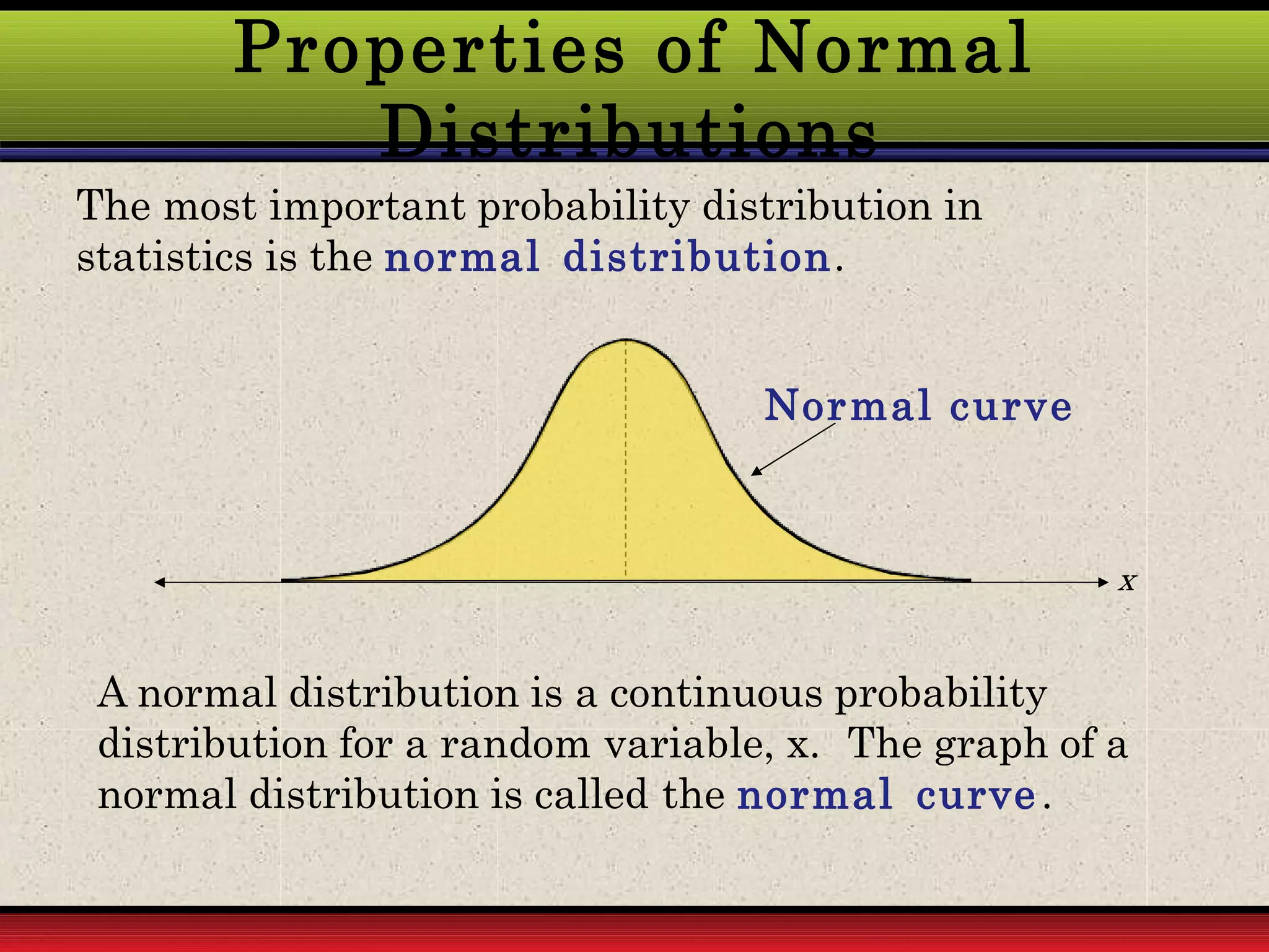
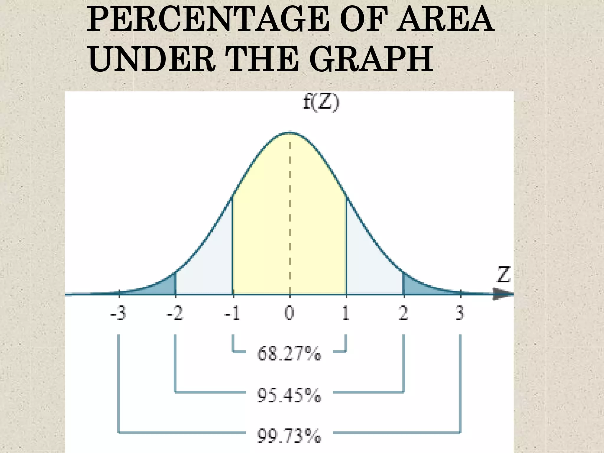
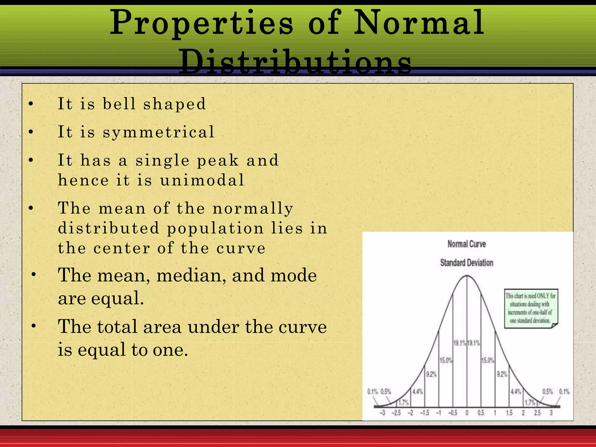
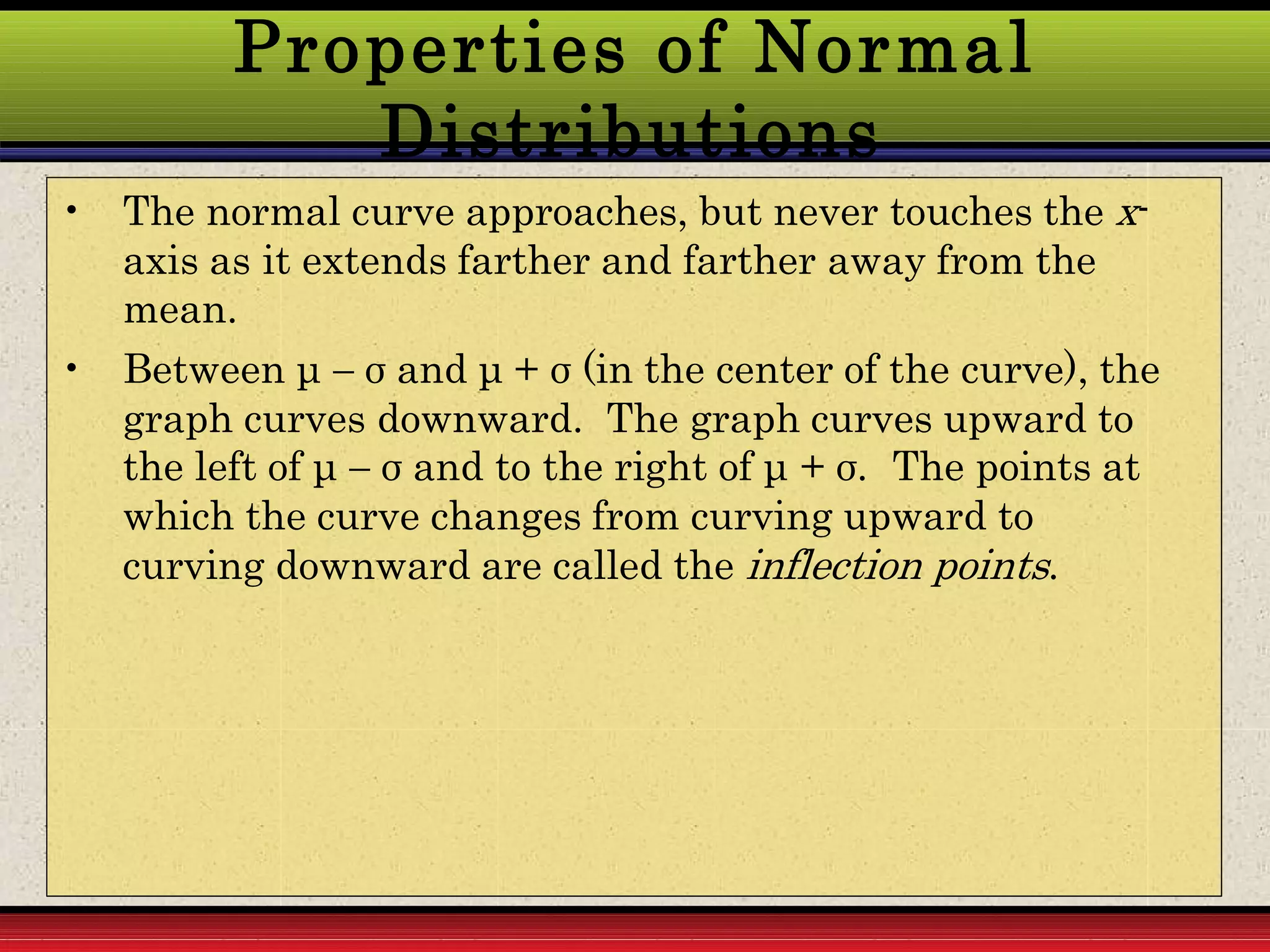
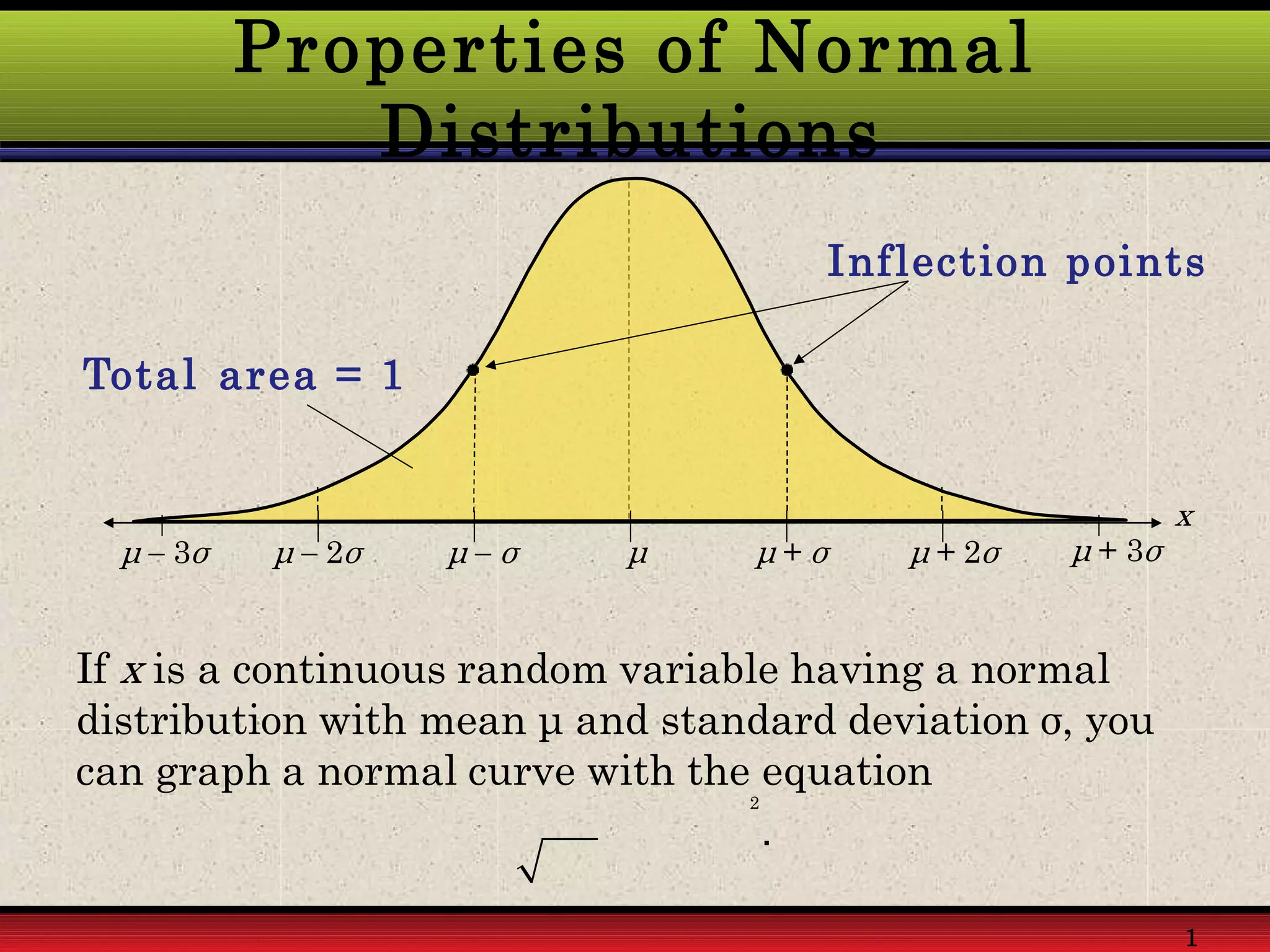
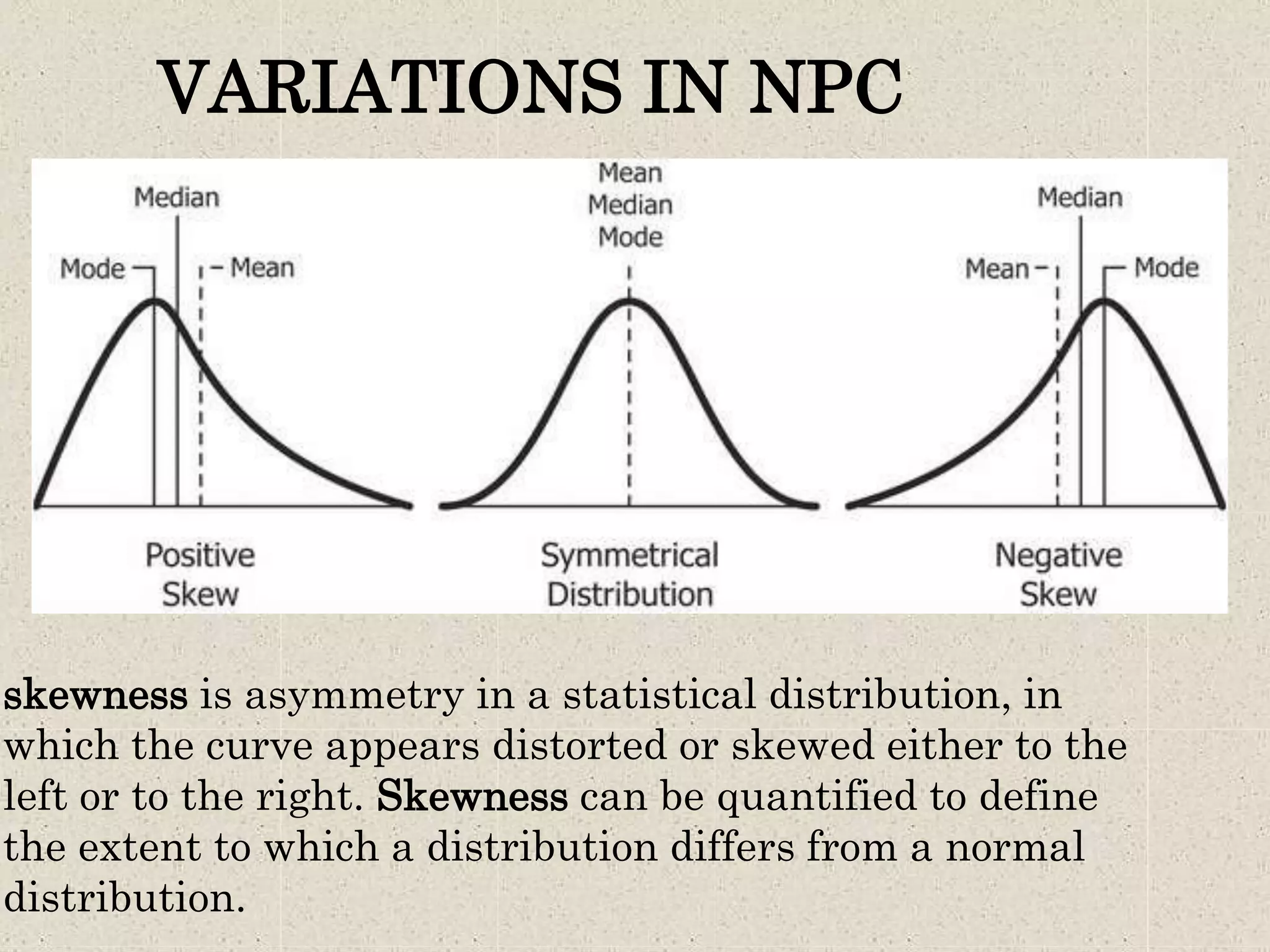
This document provides an overview of the normal probability curve. Some key points: 1. A normal probability curve, also called a normal distribution, shows how continuous data is distributed with the mean in the center. Most observations will be near the mean and fewer will be at the extremes. 2. The curve is symmetrical and bell-shaped. It has a single peak and the mean, median, and mode are equal. Half the observations are on each side of the mean. 3. The curve approaches but never touches the x-axis as it extends from the mean. Between one standard deviation of the mean, the curve curves downward, and outside it curves upward.

1. Normal
Probability
Curve
By:
Keerthi Samuel.K,
Lecturer
Vijay Marie College Of Nursing

2. • All the observations in the selected
sample should be around the mean.
This phenomena is called normal
probability or normal distribution.
• Some variables deviate from mean
which are measured by using
measures of dispersion like standard
deviation.
INTRODUCTION

3. • For individual and discreete series
poison distribution curve is used
whereas for continuous data normal
distribution is used, which is also
called normal probability distribution.
• Many statistical data in medicine are
displayed in the form of normal curve.
INTRODUCTION

4. POISSION CURVE OR BIMODAL
CURVE

5. • It was first discovered by De.Moivre as
a limitation of poison model in 1773.
• But the credit comes to Karl Gauss
who first made the reference in 1809.
NORMAL PROBABILITY CURVE

6. • When a large number of samples like
height and weight are collected, a
frequency distribution table is
prepared by keeping small class
interval. Then the features are seen as:
1. Some observations are above the mean
and some are below the mean.
2. If they are arranged in an order ,
maximum of them will be around the
mean and fewer at the extremes
PRINCIPLES

7. decreasing smoothly on both the sides.
3. Normally half the observations are
symmetrically distributed on each side of
the mean.
THE DISTRIBUTION OF THIS TYPE
OR SHAPE IS CALLED NORMAL
DISTRIBUTION OR GAUSSIAN
DISTRIBUTION
PRINCIPLES

8. Properties of Normal
Distributions
The most important probability distribution in
statistics is the normal distribution.
Normal curve
x
A normal distribution is a continuous probability
distribution for a random variable, x. The graph of a
normal distribution is called the normal curve.

9. PERCENTAGE OF AREA
UNDER THE GRAPH

10. Properties of Normal
Distributions
• It is bell shaped
• It is symmetrical
• It has a single peak and
hence it is unimodal
• The mean of the normally
distributed population lies in
the center of the curve
• The mean, median, and mode
are equal.
• The total area under the curve
is equal to one.

11. Properties of Normal
Distributions
• The normal curve approaches, but never touches the x-
axis as it extends farther and farther away from the
mean.
• Between μ  σ and μ + σ (in the center of the curve), the
graph curves downward. The graph curves upward to
the left of μ  σ and to the right of μ + σ. The points at
which the curve changes from curving upward to
curving downward are called the inflection points.

12. Properties of Normal
Distributions
μ  3σ μ + σμ  2σ μ  σ μ μ + 2σ
Inflection points
Total area = 1
If x is a continuous random variable having a normal
distribution with mean μ and standard deviation σ, you
can graph a normal curve with the equation
1
2
.
x
μ + 3σ

13. Means and Standard
Deviations
Example:
2. Which curve has the greater mean?
3. Which curve has the greater standard deviation?
The line of symmetry of curve A occurs at x = 5. The line of symmetry
of curve B occurs at x = 9. Curve B has the greater mean.
Curve B is more spread out than curve A, so curve B has the greater
standard deviation.
1 3 5 7 9 11 13
A
B
x
Larson & Farber, Elementary Statistics: Picturing the World, 3 e 1

14. Interpreting Graphs
Example:
The heights of fully grown magnolia bushes are normally
distributed. The curve represents the distribution. What
is the mean height of a fully grown magnolia bush?
Estimate the standard deviation.
The inflection points are one
standard deviation away from the
mean.
6 7 8 9 10
Height (in feet)
x
Larson & Farber, Elementary Statistics: Picturing the World, 3 e 1

15. The heights of the magnolia bushes are normally
distributed with a mean height of about 8 feet and
a standard deviation of about 0.7 feet.

16. The Standard Normal
Distribution
Larson & Farber, Elementary Statistics: Picturing the World, 3 e 16
The standard normal distribution is a normal
distribution with a mean of 0 and a standard deviation of
1.
The horizontal scale
corresponds to z-scores.
z
3 2 1 0 1 2 3
Any value can be transformed into a z-score by using the
formula z = Value - Mean = xμ- .
Standard deviation σ

17. Construction of a normal curve
• We need mean and SD . There are two methods:
 The ordinate method
 The area method
THE ORDINATE METHOD:
• Mark the midpoints to the class interval
• For each x, we find standard normal deviate the z
score.
z = Value - Mean
Standard deviation
• Find the ordinate at each of these distances from z
table
• Multiply each of these by 0.39 and take this values
frequencies corresponding to midpoints.

18. Construction of a normal curve
• THE AREA METHOD:
The tabular values of different normal deviates are
found with the help of table of areas.
The percent of area in each class is found and it is
multipled by n; the expected frequencies of each class
can be worked out.

19. VARIATIONS IN NPC
skewness is asymmetry in a statistical distribution, in
which the curve appears distorted or skewed either to the
left or to the right. Skewness can be quantified to define
the extent to which a distribution differs from a normal
distribution.

20. VARIATIONS IN NPC
Kurtosis is a statistical
measure that defines how
heavily the tails of a
distribution differ from the
tails of a normal distribution.
In other words, kurtosis
identifies whether the tails of
a given distribution contain
extreme values.