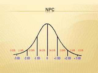
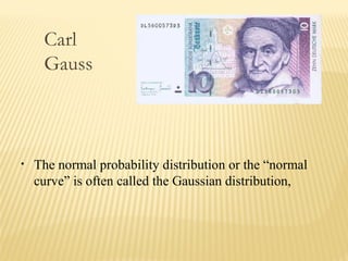
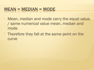
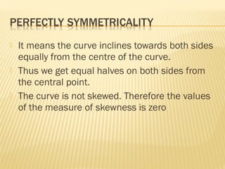
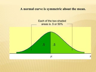
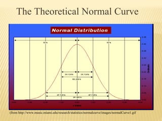
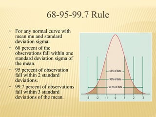
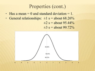
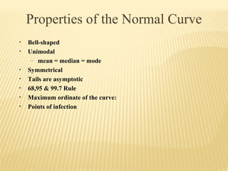
The normal distribution, also known as the Gaussian distribution, is a bell-shaped curve that is symmetric about the mean. It has three key properties: 1) the mean, median and mode have the same value and fall in the center of the curve, 2) it is perfectly symmetrical with equal areas under both halves of the curve, and 3) it extends from negative to positive infinity but almost all values lie within 3 standard deviations of the mean. The normal distribution is widely used in statistics as a model for many continuous random variables.

1. K.THIYAGU
thiyagusuri@gmail.com
surithiyagu@gmail.com

3. Carl
Gauss
• The normal probability distribution or the “normal
curve” is often called the Gaussian distribution,
Carl
Gauss

4. The shape of the curve is like that of a bell.

5.  Mean, median and mode carry the equal value.
/ same numerical value mean, median and
mode
 Therefore they fall at the same point on the
curve

6.  Since the mean , median and mode lye at one
point of the curve it is unimodal in nature.

7.  It means the curve inclines towards both sides
equally from the centre of the curve.
 Thus we get equal halves on both sides from
the central point.
 The curve is not skewed. Therefore the values
of the measure of skewness is zero

8. A normal curve is symmetric about the mean.
Each of the two shaded
areas is .5 or 50%
.5.5
μ x

9.  The curve does not touch the base or OX axis
on both sides.
 Thus it extends from negative infinity to positive
infinitive.

10.  For practical purpose the base line of the curve
is divided into six sigma distance from . Most
of the cases I.e.99.73% are covered within
such distance

11.  Maximum ordinate of the curve occurs at the
mean. I.e. where Z1=0 and the value of the
highest ordinate is 0.3989.
 The height of the ordinate at 1sigma is 0.2420
 2 sigma = 0.0540
 3 sigma = 0.0044

12. The Theoretical Normal Curve
(from http://www.music.miami.edu/research/statistics/normalcurve/images/normalCurve1.gif

13. 68-95-99.7 Rule
• For any normal curve with
mean mu and standard
deviation sigma:
• 68 percent of the
observations fall within one
standard deviation sigma of
the mean.
• 95 percent of observation
fall within 2 standard
deviations.
• 99.7 percent of observations
fall within 3 standard
deviations of the mean.

14. 68-95-99.7 Rule
997.
2
1
95.
2
1
68.
2
1
3
3
)(
2
1
2
2
)(
2
1
)(
2
1
2
2
2
=•
=•
=•
∫
∫
∫
+
−
−
−
+
−
−
−
+
−
−
−
σµ
σµ
σ
µ
σµ
σµ
σ
µ
σµ
σµ
σ
µ
πσ
πσ
πσ
dxe
dxe
dxe
x
x
x

15. Properties (cont.)
• Has a mean = 0 and standard deviation = 1.
• General relationships: ±1 s = about 68.26%
±2 s = about 95.44%
±3 s = about 99.72%
-5 -4 -3 -2 -1 0 1 2 3 4 5
68.26%
95.44%
99.72%

16.  The scale values are analysed as
Z1=(X-M)/sigma
Where z1 = 0 and range of mean plus or minus Z is
equal to mean plus or minus sigma

17.  The points of infection are each plus or minus
one sigma from above and below the mean.
 The curve changes from convex to concave at
these points with the baseline.

18. Various measures
In the normal curve
 Quartile deviation Q = Proper error = 0.6745a
 Mean deviation, AD = 0.7979a
 Skewness = 0
 Kurtosis = 0.263

19. Properties of the Normal Curve
• Bell-shaped
• Unimodal
– mean = median = mode
• Symmetrical
• Tails are asymptotic
• 68,95 & 99.7 Rule
• Maximum ordinate of the curve:
• Points of infection

20. APPLICATIONS OF THE NORMAL PROBABILITY CURVE
To normalize a frequency distribution. It is an important step in standardizing a
psychological test or inventory.
To test the significance of observations in experiments, findings them
relationships with the chance fluctuations or errors that are result of sampling
procedures.
To generalize about population from which the samples are drawn by calculating
the standard error of mean and other statistics.
To compare two distributions. The NPC is used to compare two distributions.
To determine the difficulty values. The Z scores are used to determine the
difficulty values of test items.
To classify the groups. The Normal Probability Curve (NPC) is used for
classifying the groups and assigning grades to individuals.
To determine the level of significance. The levels of significance of statistics
results are determined in terms of NPC limits.
To scale responses to opinionnaires, judgement, ratings or rankings by
transforming them numerical values.

22.  Skewness means asymmetrial nature.
 When the curve on clones towards right or left
we cannot take it as a normal curve but as a
skewed curve.
 The degree of departure from symmetry is
called symmetry.

23. Skewness
 Positive Skewness: Mean ≥ Median
 Negative Skewness: Median ≥ Mean
 Pearson’s Coefficient of Skewness3
:
= 3 (Mean –Median)
Standard deviation

24.  When the curve inclines more to the left
skewness becomes negative
m
ean
m
edian
m
ode
Negative or Left Skew Distribution

25.  When the curve inclines more towards right
m
ean
m
edian
m
ode
Positive or Right Skew Distribution

26. C.I.
NORMAL CURVE POSITIVELY
SKEWED
NEGATIVELY
SKEWED
f f f
91 - 100 2 2 20
81 – 90 3 2 10
71 - 80 10 3 10
61 – 70 20 3 3
51 – 60 10 10 3
41 – 50 3 10 2
31 - 40 2 20 2

27. Reason

28.  Literally kurtosis means tendency of ‘flatness’
or ‘peakedness’.
 The normal curve is moderately peaked.

29. kurtosis: the proportion of a curve located in the
center, shoulders and tails
How fat or thin the tails are
leptokurtic
no shoulders
platykurtic
wide shoulders

30.  When the curve is more flattened the
distribution will be called as platy kurtoc

31.  When the curve is more peaked than normal
one it is called as lepto kurtoc curve

32. 1090 PP
Q
Ku
−
=
Where Q = quartile deviation,
P90 = 90th
percentile
P10 = 10th
percentile

33.  Biased selection of sample
 Scoring errors
 Improper construction of a test
 Improper administration of a test
 Abnormality in the traits of the items.