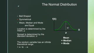
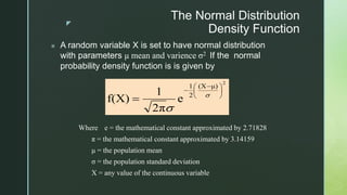
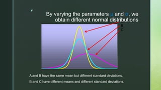
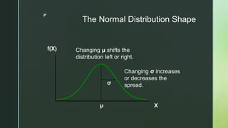
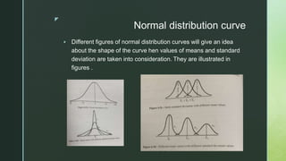
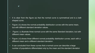
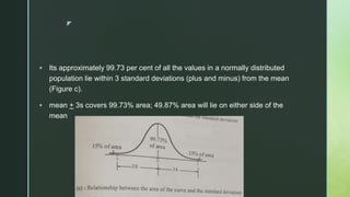
The document provides an overview of the normal distribution, highlighting its characteristics such as symmetry, bell shape, and the equality of mean, median, and mode. It explains how any normal distribution can be standardized to the z distribution with a mean of 0 and a standard deviation of 1, and discusses the significance of the normal distribution in statistical analysis, especially with large sample sizes. Additionally, it outlines properties of the normal curve and the distribution of data within standard deviations from the mean.

1. z
Normal
Distribution

2. z
Continuous Probability Distributions
 A continuous variable is a variable that can assume any value on a
continuum (can assume an uncountable number of values)
 thickness of an item
 time required to complete a task
 temperature of a solution
 height, in inches
 These can potentially take on any value depending only on the ability to
precisely and accurately measure

3. z
 Bell Shaped
 Symmetrical
 Mean, Median and Mode
are Equal
Location is determined by the
mean, μ
Spread is determined by the
standard deviation, σ
The random variable has an infinite
theoretical range:
+  to  
Mean
= Median
= Mode
X
f(X)
μ
σ
The Normal Distribution

4. z
The Normal Distribution
Density Function
2
μ)
(X
2
1
e
2π
1
f(X)





 

 

 A random variable X is set to have normal distribution
with parameters μ mean and varience σ2 If the normal
probability density function is is given by
Where e = the mathematical constant approximated by 2.71828
π = the mathematical constant approximated by 3.14159
μ = the population mean
σ = the population standard deviation
X = any value of the continuous variable

5. z
A
B
C
A and B have the same mean but different standard deviations.
B and C have different means and different standard deviations.
By varying the parameters μ and σ, we
obtain different normal distributions

6. z
The Normal Distribution Shape
X
f(X)
μ
σ
Changing μ shifts the
distribution left or right.
Changing σ increases
or decreases the
spread.

7. z
The Standardized Normal
 Any normal distribution (with any mean and standard deviation
combination) can be transformed into the standardized normal
distribution (Z)
 To compute normal probabilities need to transform X units
into Z units
 The standardized normal distribution (Z) has a mean of 0 and
a standard deviation of 1

8. z
Translation to the Standardized Normal
Distribution
 Translate from X to the standardized normal (the “Z”
distribution) by subtracting the mean of X and dividing by its
standard deviation:
σ
μ
X
Z


The Z distribution always has mean = 0 and
standard deviation = 1

9. z
The Standardized Normal Probability
Density Function
 The formula for the standardized normal probability density
function is
Where e = the mathematical constant approximated by 2.71828
π = the mathematical constant approximated by 3.14159
Z = any value of the standardized normal distribution
2
(1/2)Z
e
2π
1
f(Z) 


10. z
The Standardized
Normal Distribution
Also known as the “Z” distribution
Mean is 0
Standard Deviation is 1
Z
f(Z)
0
1
Values above the mean have positive Z-values.
Values below the mean have negative Z-values.

11. z
Importance of normal distribution
Importance of the normal distribution
The importance of normal distribution would be clear from the following points:
1. In most of the biological analyses, values are often distributed in accordance with
the normal distribution. As the sample size increases, the distribution of mean of a
random sample approaches a normal distribution. On the other hand, if the samples
of the large size are drawn from a population which is not normally distributed, the
successive sample means will form normal distribution. A small sample shows an
irregular distribution due to obvious error in the sample. However, large sample size
will reduce the error and make the curve smooth.
2. When the size of the samples becomes large, the normal distribution serves as a
good approximation of discrete distribution such as Binomial and Poison.

12. z
Properties of the normal distribution
The normal distribution curve has the following properties:
 The normal curve is "bell-shaped" and is symmetrical in appearance. It has a single peak,
thus it is unimodal.
 The mean of a normally distributed population lies at the centre of its normal curve. The
height of the normal curve is at its maximum at the mean. This ordinate divides the curve in
two equal parts.
 The mean, median and mode are all equal in normal distribution.
 The height of the curve declines on either side of the peak which occurs at the mean.
 The area on both the sides of the peak is equal to each other.
 The curve is asymptotic to the base on either side. The two tails never touch the base line.

13. z
Normal distribution curve
 Different figures of normal distribution curves will give an idea
about the shape of the curve hen values of means and standard
deviation are taken into consideration. They are illustrated in
figures .

14. z
 It is clear from the figure (a) that the normal curve is symmetrical and is a bell-
shaped curve.
 Figure ( b) shows the normal probability distribution curves with the same mean,
but with different standard deviation values.
 Figure ( c) illustrate three normal curve with the same Standard deviation, but with
different mean values.
 Figure ( d) shows three different normal probability distribution curves, each with a
different mean and a different standard deviation.
 It can concluded from these curves that a normal curve can describe a large
number of populations differentiated only by the mean and the standard deviation

15. z
Area under normal distribution
The area under normal curve is distributed as follows :
 It is approximately 68 per cent of all the values in a normally distributed
population that lie within 1 standard deviation (plus and minus) from the
mean (Figure a). Mean + 1s covers 68.27% area; 34.14% area will lie on
either side of the mean.

16. z
 It is approximately 95.45 per cent of all the values in a normally distributed
population that lie within 2 standard deviation (plus and minus) from the mean
(Figure b).
 × + 2s covers 95.45% area; 47.73% area will lie on either side of the mean.

17. z
 Its approximately 99.73 per cent of all the values in a normally distributed
population lie within 3 standard deviations (plus and minus) from the mean
(Figure c).
 mean + 3s covers 99.73% area; 49.87% area will lie on either side of the
mean

18. z

19. z

20. z

21. z

22. z
THANK YOU