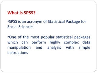
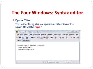
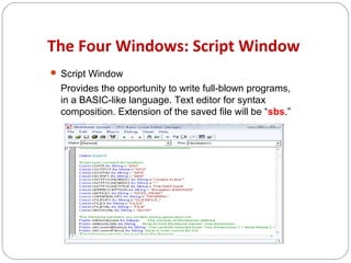
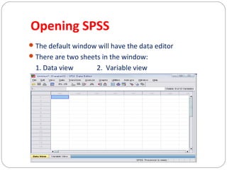
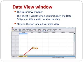
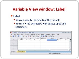
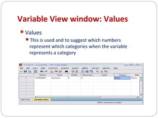
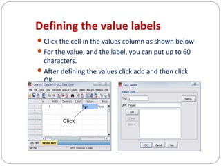
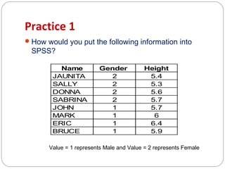
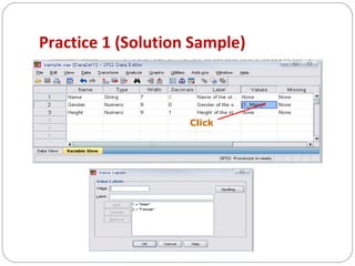
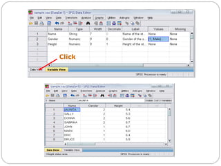
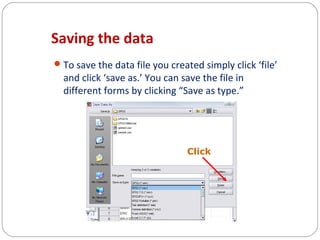
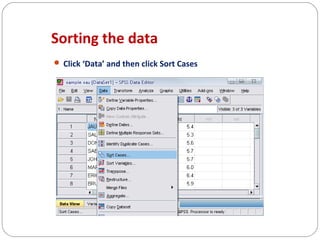
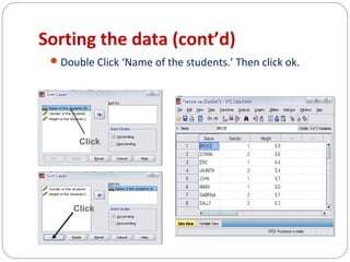
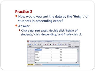
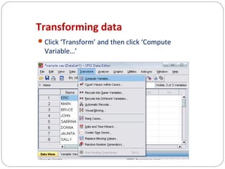
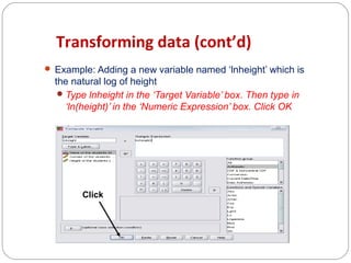
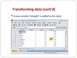
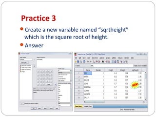
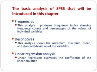
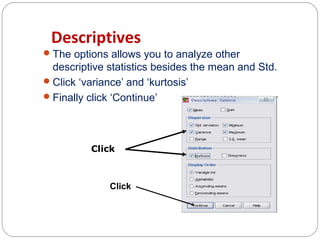
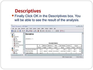
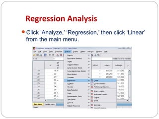
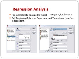
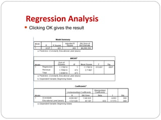
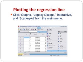
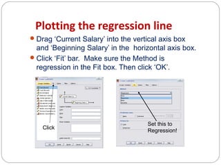
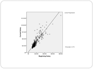
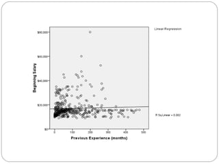
This document provides an overview of the Statistical Package for Social Sciences (SPSS). It discusses what SPSS is, how to define and enter variables, and the four main windows in SPSS including the data editor, output viewer, syntax editor, and script window. Basic functions like frequencies analysis, descriptives, and linear regression are also introduced.

1. Two-day workshop on Frontier areas in
Symbolic Computing and Cloud Computing
A TRAINING PROGRAMME ON SOFTWARE
PACKAGES FOR STATISTICAL ANALYSIS (SPSS)
Day 1 – Session 2
By
B. Anand
Network Engineer
Bharathidasan University

2. What is SPSS?
•SPSS is an acronym of Statistical Package for
Social Sciences
•One of the most popular statistical packages
which can perform highly complex data
manipulation and analysis with simple
instructions

3. What is SPSS?
•SPSS is an acronym of Statistical Package for
Social Sciences
•One of the most popular statistical packages
which can perform highly complex data
manipulation and analysis with simple
instructions

4. Variable
Variable is the name of the field in the
dataset.
Data
Data is the value given to the field.
Measuring the Variables
Ordinal - region, zip code, or religious affiliation
Nominal - Levels of service satisfaction from highly dissatisfied
to highly satisfied
Scale -
age in years and income in thousands of dollars

5. The Four Windows:
• Data editor
• Output viewer
• Syntax editor
• Script window

6. The Four Windows: Data Editor
 Data Editor
Spreadsheet-like system for defining, entering, editing,
and displaying data.
Extension of the saved file will be “sav.”

7. The Four Windows: Output Viewer
 Output Viewer
Displays output and errors. Extension of the saved file will
be “spv.”

8. The Four Windows: Syntax editor
 Syntax Editor
Text editor for syntax composition. Extension of the
saved file will be “sps.”

9. The Four Windows: Script Window
 Script Window
Provides the opportunity to write full-blown programs,
in a BASIC-like language. Text editor for syntax
composition. Extension of the saved file will be “sbs.”

10. Opening SPSS
 The default window will have the data editor
 There are two sheets in the window:
1. Data view
2. Variable view

11. Data View window
 The Data View window
This sheet is visible when you first open the Data
Editor and this sheet contains the data
 Click on the tab labeled Variable View
Click

12. Variable View window
 This sheet contains information about the data set that is stored
with the dataset
 Name
 The first character of the variable name must be alphabetic
 Variable names must be unique, and have to be less than 64
characters.
 Spaces are NOT allowed.

13. Variable View window: Type
 Type
Click on the ‘type’ box. The two basic types of variables
that you will use are numeric and string. This column
enables you to specify the type of variable.

14. Variable View window: Width
 Width
Width allows you to determine the number of
characters SPSS will allow to be entered for the
variable

15. Variable View window: Decimals
Decimals
Number of decimals
It has to be less than or equal to 16
3.14159265

16. Variable View window: Label
Label
You can specify the details of the variable
You can write characters with spaces up to 256
characters

17. Variable View window: Values
Values
This is used and to suggest which numbers
represent which categories when the variable
represents a category

18. Defining the value labels
 Click the cell in the values column as shown below
 For the value, and the label, you can put up to 60
characters.
 After defining the values click add and then click
OK.
Click

19. Practice 1
 How would you put the following information into
SPSS?
Name
JAUNITA
SALLY
DONNA
SABRINA
JOHN
MARK
ERIC
BRUCE
Gender
2
2
2
2
1
1
1
1
Height
5.4
5.3
5.6
5.7
5.7
6
6.4
5.9
Value = 1 represents Male and Value = 2 represents Female

20. Practice 1 (Solution Sample)
Click

21. Click

22. Saving the data
 To save the data file you created simply click ‘file’
and click ‘save as.’ You can save the file in
different forms by clicking “Save as type.”
Click

23. Sorting the data
 Click ‘Data’ and then click Sort Cases

24. Sorting the data (cont’d)
 Double Click ‘Name of the students.’ Then click ok.
Click
Click

25. Practice 2
How would you sort the data by the ‘Height’ of
students in descending order?
Answer
Click data, sort cases, double click ‘height of
students,’ click ‘descending,’ and finally click ok.

26. Transforming data
 Click ‘Transform’ and then click ‘Compute
Variable…’

27. Transforming data (cont’d)
 Example: Adding a new variable named ‘lnheight’ which is
the natural log of height
 Type lnheight in the ‘Target Variable’ box. Then type in
‘ln(height)’ in the ‘Numeric Expression’ box. Click OK
Click

28. Transforming data (cont’d)
 A new variable ‘lnheight’ is added to the table

29. Practice 3
Create a new variable named “sqrtheight”
which is the square root of height.
Answer

30. The basic analysis

31. The basic analysis of SPSS that will be
introduced in this chapter
Frequencies
This analysis
produces frequency tables showing
frequency counts and percentages of the values of
individual variables.
Descriptives
This analysis shows the maximum, minimum, mean,
and standard deviation of the variables
Linear regression analysis
Linear Regression estimates the coefficients of the
linear equation

32. Opening the sample data
 Open ‘Employee data.sav’ from the SPSS
 Go to “File,” “Open,” and Click Data

33. Opening the sample data
 Go to Program Files,” “SPSSInc,” “SPSS17,” and
“Samples” folder.
 Open “Employee Data.sav” file

34. Frequencies
 Click ‘Analyze,’ ‘Descriptive statistics,’ then
click ‘Frequencies’

35. Frequencies
Click gender and put it into the variable box.
Click ‘Charts.’
Then click ‘Bar charts’ and click ‘Continue.’
Click
Click

36. Frequencies
Finally Click OK in the Frequencies box.
Click

38. Using the Syntax editor
Click ‘Analyze,’ ‘Descriptive statistics,’ then
click ‘Frequencies.’
Put ‘Gender’ in the Variable(s) box.
Then click ‘Charts,’ ‘Bar charts,’ and click
‘Continue.’
Click ‘Paste.’
Click

39. Using the Syntax editor
Highlight the commands in the Syntax
editor and then click the run icon.
You can do the same thing by right clicking
the highlighted area and then by clicking
‘Run Current’
Click
Right
Click!

40. Practice 4
Do a frequency analysis on the variable
“minority”
Create pie charts for it
Do the same analysis using the syntax editor

42. Answer
Click

43. Descriptives
Click ‘Analyze,’ ‘Descriptive statistics,’ then
click ‘Descriptives…’
Click ‘Educational level’ and ‘Beginning
Salary,’ and put it into the variable box.
Click Options
Click

44. Descriptives
 The options allows you to analyze other
descriptive statistics besides the mean and Std.
 Click ‘variance’ and ‘kurtosis’
 Finally click ‘Continue’
Click
Click

45. Descriptives
Finally Click OK in the Descriptives box. You
will be able to see the result of the analysis.

46. Regression Analysis
Click ‘Analyze,’ ‘Regression,’ then click ‘Linear’
from the main menu.

47. Regression Analysis
 For example let’s analyze the model
salbegin = β 0 + β1edu + ε
 Put ‘Beginning Salary’ as Dependent and ‘Educational Level’ as
Independent.
Click
Click

48. Regression Analysis
 Clicking OK gives the result

49. Plotting the regression line
Click ‘Graphs,’ ‘Legacy Dialogs,’ ‘Interactive,’
and ‘Scatterplot’ from the main menu.

50. Plotting the regression line
 Drag ‘Current Salary’ into the vertical axis box
and ‘Beginning Salary’ in the horizontal axis box.
 Click ‘Fit’ bar. Make sure the Method is
regression in the Fit box. Then click ‘OK’.
Click
Set this to
Regression!

52. Practice 5
Find out whether or not the previous experience
of workers has any affect on their beginning
salary?
Take the variable “salbegin,” and “prevexp” as dependent and
independent variables respectively.
Plot the regression line for the above analysis
using the “scatter plot” menu.

53. Answer
Click

55. Click on the “fit” tab to make
sure the method is regression