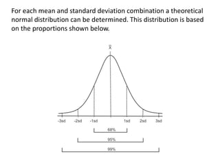
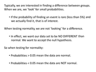
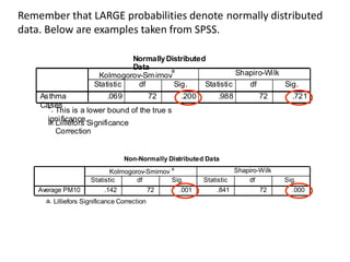
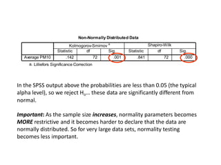
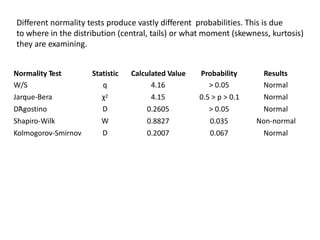
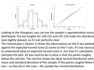
This document discusses testing for normality in statistical data. It describes comparing an actual data distribution to a theoretical normal distribution based on the data's mean and standard deviation. Several graphical and statistical tests for normality are presented, including Q-Q plots, Kolmogorov-Smirnov tests, and Shapiro-Wilk tests. Large p-values from these tests indicate the data are normally distributed, while small p-values show the data are non-normal. The document emphasizes that normality testing is more important for smaller sample sizes and provides guidelines for selecting an appropriate normality test.

1. Testing for Normality

2. For each mean and standard deviation combination a theoretical
normal distribution can be determined. This distribution is based
on the proportions shown below.

3. This theoretical normal distribution can then be compared to the
actual distribution of the data.
The actual data
distribution that has a
mean of 66.51 and a
standard deviation of
18.265.
Theoretical normal
distribution calculated
from a mean of 66.51 and a
standard deviation of
18.265.
Are the actual data statistically different than the computed
normal curve?

4. There are several methods of assessing whether data are
normally distributed or not. They fall into two broad categories:
graphical and statistical. The some common techniques are:
Graphical
• Q-Q probability plots
• Cumulative frequency (P-P) plots
Statistical
•
•
•
•
•
Jarque-Bera test
Shapiro-Wilks test
Kolmogorov-Smirnov test
D’
Agostino test

5. Q-Q plots display the observed values against normally
distributed data (represented by the line).
Normally distributed data fall along the line.

6. Graphical methods are typically not very useful when the sample size is
small. This is a histogram of the last example. These data do not ‘look’
normal, but they are not statistically different than normal.

7. Tests of Normality
a. Lilliefors Significance Correction
Tests of Normality
a. Lilliefors Significance Correction
Tests of Normality
*. This is a lower bound of the true significance.
a. Lilliefors Significance Correction
a
Kolmogorov-Smirnov Shapiro-Wilk
Statistic df Sig. Statistic df Sig.
Z100 .071 100 .200* .985 100 .333
a
Kolmogorov-Sm irnov Shapiro-Wi lk
Statisti c df Sig. Statisti c df Sig.
TOTAL_VALU .283 149 .000 .463 149 .000
a
Kolmogorov-Smirnov Shapiro-Wilk
Statistic df Sig. Statistic df Sig.
Age .110 1048 .000 .931 1048 .000

8. Statistical tests for normality are more precise since actual
probabilities are calculated.
Tests for normality calculate the probability that the sample
drawn from a normal population.
was
The hypotheses used are:
Ho: The sample data are not significantly
normal population.
different than a
Ha: The sample data are significantly different than a normal
population.

9. Typically, we are interested in finding a difference between groups.
When we are, we ‘look’ for small probabilities.
• If the probability of finding an event is rare (less than 5%)
we actually find it, that is of interest.
and
When testing normality, we are not ‘looking’ for a difference.
• In effect, we want our data set to be NO DIFFERENT
normal. We want to accept the null hypothesis.
than
So when testing for normality:
• Probabilities > 0.05 mean the data are normal.
• Probabilities < 0.05 mean the data are NOT normal.

10. Remember that LARGE probabilities denote normally distributed
data. Below are examples taken from SPSS.
NormallyDistributed
Data
*. This is a lower bound of the true s
ignificance.
a.Lilliefors Significance
Correction
Non-Normally Distributed Data
a. Lilliefors Significance Correction
Kolmogorov-Smirnov
a Shapiro-Wilk
Statistic df Sig. Statistic df Sig.
Average PM10 .142 72 .001 .841 72 .000
a
Kolmogorov-Sm irnov Shapiro-Wilk
Statistic df Sig. Statistic df Sig.
Asthma
Cases
.069 72 .200
*
.988 72 .721

11. NormallyDistributed
Data
*. This is a lower bound of the true s
ignificance.
a.Lilliefors Significance
Correction
In SPSS output above the probabilities are greater than 0.05 (the
typical alpha level), so we accept Ho… these data are not different
from normal.
a
Kolmogorov-Sm irnov Shapiro-Wilk
Statistic df Sig. Statistic df Sig.
Asthma
Cases
.069 72 .200
*
.988 72 .721

12. Non-Normally Distributed Data
a. Lilliefors Significance Correction
In the SPSS output above the probabilities are less than 0.05 (the typical
alpha level), so we reject Ho… these data are significantly different from
normal.
Important: As the sample size increases, normality parameters becomes
MORE restrictive and it becomes harder to declare that the data are
normally distributed. So for very large data sets, normality testing
becomes less important.
Kolmogorov-Smirnov
a Shapiro-Wilk
Statistic df Sig. Statistic df Sig.
Average PM10 .142 72 .001 .841 72 .000

13. Jarque–Bera Test
A goodness-of-fit test of whether sample data have the skewness
and kurtosis matching a normal distribution.
n n
 
x)3
(x  x)4
(x 
i i
i1 i1
k  k4  3
3
ns3
ns4
k3

k4

2 2
 
n 
JB  
 
6 24
 
Where x is each observation, n is the sample size, s is the
standard deviation, k3 is skewness, and k4 is kurtosis.

14. D’Agostino Test
• A very powerful test for departures from normality.
• Based on
value.
the D statistic, which gives an upper and lower critical
n  1
T 
T   i

D  where X i
2
3
 
n SS
where D is the test statistic, SS is the sum of squares of the data
and n is the sample size, and i is the order or rank of observation
X. The df for this test is n (sample size).
• First the data are ordered from smallest to largest or largest to
smallest.

15. Different normality tests produce vastly different probabilities. This is due
to where in the distribution (central, tails) or what moment (skewness, kurtosis)
they are examining.
Normality Test
W/S
Jarque-Bera
D’
Agostino
Shapiro-Wilk
Kolmogorov-Smirnov
Statistic
q
χ2
D
W
D
Calculated Value
4.16
4.15
0.2605
0.8827
0.2007
Probability
> 0.05
0.5 > p > 0.1
> 0.05
0.035
0.067
Results
Normal
Normal
Normal
Non-normal
Normal

16. Which normality test should I use?
Kolmogorov-Smirnov:
• Not sensitive to problems in the tails.
• For data sets > 50.
Shapiro-Wilks:
• Doesn't work well if several values in the data set are the same.
• Works best for data sets with < 50, but can be used with larger
data sets.
W/S:
• Simple, but effective.
• Not available in SPSS.
Jarque-Bera:
• Tests for skewness and kurtosis, very effective.
• Not available in SPSS.
D’Agostino:
• Powerful omnibus (skewness, kurtosis, centrality) test.
• Not available in SPSS.

17. When is non-normality a problem?
• Normality can be a problem when the sample size is small (< 50).
• Highly skewed data create problems.
• Highly leptokurtic data are problematic, but not as much as
skewed data.
• Normality becomes a serious concern when there is “activity”
the tails of the data set.
in
• Outliers are a problem.
• “Clumps” of data in the tails are worse.

18. Final Words Concerning Normality Testing:
1. Since it IS a test, state a null and alternate hypothesis.
2. If you perform a normality test, do not ignore the results.
3. If the data are not normal, use non-parametric tests.
4. If the data are normal, use parametric tests.
AND MOST IMPORTANTLY:
5. If you have groups of data, you MUST test each group
normality.
for

19. Variations on the normal plot
Quantile is just another word for a normal or Z-score and refers to
what’s shown on the Y axis .There are actually four variations of the
normal plot, or eight since depending on preference the X and Y
axes are often swapped:
Normal quantile plot.
Observations plotted against expected normal score (Z-score,
known as quantiles)
Normal quantile-quantile plot (also known as normal QQ plot).
Normal score (Z-score, known as quantiles) of the observations
plotted against expected normal score (Z-score, known as
quantiles)

20. Normal probability plot.
Observations plotted against expected CDF (cumulative area
under the normal curve, known as probability)
Normal probability-probability plot (also known as normal PP
plot).
CDF (cumulative area under the normal curve, known as
probability) of the observations plotted against expected CDF
(cumulative area under the normal curve, known as probability)

21. By their nature, normal plots based on probability fail to emphasize
non-normality in extreme observations – in the tails of the
distribution – as well as quantile based normal plots. Generally,
probability/P-P plots are better to spot non-normality around the
mean, and normal quantile/Q-Q plots to spot non-normality in the
tails.
Thankfully, whichever of variation of the normal plot you’re faced
with, interpretation is the same. If the sample is normal you should
see the points roughly follow a straight-line.
In future posts we’ll show cases of skewed and peaked
distributions, and explain how you can identify these problems
from the histogram and normal plot.

22. Looking at the histogram, you can see the sample is approximately norma
distributed. The bar heights for 120-122 and 122-124 make the distributio
look slightly skewed, so it’s not perfectly clear.
The normal plot is clearer. It shows the observations on the X axis plotted
against the expected normal score (Z-score) on the Y axis. It’s not necessa
to understand what an expected normal score is, nor how it’s calculated, t
interpret the plot. All you need to do is check is that the points roughly
follow the red-line. The red-line shows the ideal normal distribution with
mean and standard-deviation of the sample. If the points roughly follow t
line – as they do in this case – the sample has normal distribution.