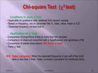
This document discusses various statistical concepts such as measures of central tendency, measures of dispersion, standard deviation, normal distribution, and tests of significance. It provides examples and formulas to calculate range, mean deviation, standard deviation, z-scores, confidence intervals, and the chi-square test. Biological variation is common and various statistical methods can be used to analyze data and find patterns in large datasets.

1. Biological variation in large groups is common. e.g : BP, wt What is normal variation? and How to measure? Measure of dispersion helps to find how individual observations are dispersed around the central tendency of a large series Deviation = Observation - Mean 10/01/11 STATISTICS

2. Range Quartile deviation Mean deviation Standard deviation Variance Coefficient of variance : indicates relative variability ( SD/Mean) x100 10/01/11 STATISTICS

3. Range : difference between the highest and the lowest value Problem: Systolic and diastolic pressure of 10 medical students are as follows: 140/70, 120/88, 160/90, 140/80, 110/70, 90/60, 124/64, 100/62, 110/70 & 154/90. Find out the range of systolic and diastolic blood pressure Solution: Range of systolic blood pressure of medical students: 90-160 or 70 Range of diastolic blood pressure of medical students: 60-90 or 30 Mean Deviation: average deviations of observations from mean value _ Σ (X – X ) __ Mean deviation (M.D) = --------------- , ( where X = observation, X = Mean n n= number of observation ) 10/01/11 STATISTICS

4. Problem : Find out the mean deviation of incubation period of measles of 7 children, which are as follows: 10, 9, 11, 7, 8, 9, 9. Solution: Mean deviation (MD ) = _ Σ X - X = ------------ n = 6 / 7 = 0.85 10/01/11 STATISTICS Observation (X) __ Mean ( X ) __ Deviation (X - X) 10 __ X = Σ X / n = 63 / 7 = 9 1 9 0 11 2 7 -2 8 -1 9 0 9 0 ΣX=63 _ Σ (X-X) = 6, ignoring + or - signs

5. It is the most frequently used measure of dispersion S.D is the Root-Means-Square-Deviation S.D is denoted by σ or S.D ___________ Σ ( X – X ) 2 S.D (σ) = γ ---------------------- n 10/01/11 STATISTICS

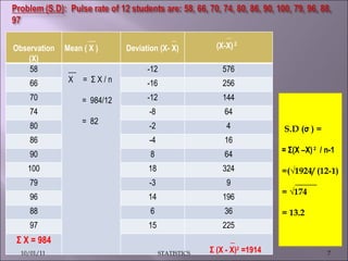
6. Calculate the mean ↓ Calculate difference between each observation and mean ↓ Square the differences ↓ Sum the squared values ↓ Divide the sum of squares by the no. observations (n) to get ‘mean square deviation’ or variances (σ 2 ) . [For sample size < 30, it will be divided by (n-1)] ↓ Find the square root of variance to get Root-Means-Square-Deviation or S.D ( σ) 10/01/11 STATISTICS

7. S.D ( σ ) = = Σ(X –X) 2 / n-1 =(√1924/ (12-1) _____ = √174 = 13.2 10/01/11 STATISTICS Observation (X) __ Mean ( X ) _ Deviation (X- X) __ (X-X) 2 58 __ X = Σ X / n = 984/12 = 82 -12 576 66 -16 256 70 -12 144 74 -8 64 80 -2 4 86 -4 16 90 8 64 100 18 324 79 -3 9 96 14 196 88 6 36 97 15 225 Σ X = 984 _ Σ (X - X) 2 =1914

8. x The Empirical Rule (applies to bell-shaped distributions ) FIGURE 2-15 10/01/11 STATISTICS

9. x - s x x + s 68% within 1 standard deviation 34% 34% The Empirical Rule (applies to bell-shaped distributions ) FIGURE 2-15 10/01/11 STATISTICS

10. x - 2s x - s x x + 2s x + s 68% within 1 standard deviation 34% 34% 95% within 2 standard deviations The Empirical Rule (applies to bell-shaped distributions ) 13.5% 13.5% FIGURE 2-15 10/01/11 STATISTICS

11. x - 3s x - 2s x - s x x + 2s x + 3s x + s 68% within 1 standard deviation 34% 34% 95% within 2 standard deviations 99.7% of data are within 3 standard deviations of the mean The Empirical Rule (applies to bell-shaped distributions ) 0.1% 2.4% 2.4% 13.5% 13.5% FIGURE 2-15 10/01/11 STATISTICS 0.1%

12. Other names : Frequency distribution curve, Normal curve, Gaussian Curve etc. Most of the biological variables (continuous) follow normal distribution Applicable for quantitative data (when large no. of observations) Quantitative data - represented by a histogram & by joining midpoints of each rectangle in the histogram we can get a frequency polygon When number of observations become very large and class interval very much reduced, the frequency polygon loses its angulations and gives rise to a smooth curve known as frequency curve. 10/01/11 STATISTICS

13. Mean  1 SD limit, includes 68.27% of all the observations Mean  1.96 SD limit, includes 95% of all observations Mean  2 SD limit, includes 95.45% of all observations Mean  2.58 SD limit, includes 99% of all observations Mean  3 SD limit, includes 99.73% of all observations 10/01/11 STATISTICS

14. Observations of a continuous variable, those are normally distributed in a popln., when plotted as a frequency curve give rise to Normal Curve The characteristics of Normal Curve: - A smooth bell shaped symmetrical curve - A area under the curve is 1 or 100%. - Mean, median and mode - identical (at same point). - Never touch the base line. - Limit on either side is called ‘ Confidence limit’. - Curve tells the probability of occurrence by chance (sample variability) or how many times an observation can occur normally in the popln. - Distribution of observations under normal curve follows the same pattern of Normal Distribution 10/01/11 STATISTICS

15. Each observation under a normal curve has a ‘Z’ value Z (standard normal variate or relative deviate or critical ratio) is the measure of distance of the observation from mean in terms of standard deviation __ Z=(Observation-Mean)/S.D=( X - X ) / S.D So, if ‘Z’ score is – 2, it means that the observation is 2 S.D away from mean on left hand side. Similarly, Z is + 2, it means that the observation is 2 S.D away from mean on right hand side. When ‘Z’ score is expressed in terms of absolute value, suppose, 2, it means that the observation is 2 S.D away from mean irrespective of the direction. If all observations of normal curves are replaced by ‘Z’ score, virtually all curves become the same. This standardized curve is known as STANDARD NORMAL CURVE 10/01/11 STATISTICS

16. Properties : - All properties of Normal Curve - Area under the curve is 1 - Mean, median & mode coincide and they are 0 - Standard deviation is 1 The Standard Normal Curve and Areas within 1, 2, 3 SD's of the Mean 10/01/11 STATISTICS

17. Areas within 1 & 2 S.D's of the Mean ( Mean-36, SD-8) and (Mean-70, SD-3) 10/01/11 STATISTICS

18. The confidence level or reliability is the expected percentage of times that the actual values will fall within the stated precision limit. Thus 95 % CI mean that there are 95 chances in 100 (or 0.95 in 1) that the sample results represent the true condition of population within a specified precision range against 5 chances in 100 (0.05 in 1) that it does not. Precision is the range within which the answer may vary and still be accepted CI indicates the chance that the answer will fall within that range & Significance level indicates the likelihood that the answer will fall outside that range We always remember that if the confidence level is 95%, then the significance level will be (100-95) i.e., 5%; if the confidence level is 99%, significance level is (100-99) i.e.,1% Area of normal curve within precision limits for the specified CI constitutes the accepted zone and area of curve outside this limit in either direction constitutes the rejection zone. 10/01/11 STATISTICS

19. __ __ CI= Mean ± Z SE (Mean) = X ± Z SE (X) _ _ 95% CI = X ± 1.96 SE (X) _ _ 99% CI = X ± 2.58 SE (X ) 10/01/11 STATISTICS

20. Large sample- sample size > 30 Small sample- sample size > 30 Hypothesis – Null ( H 0 )- assumes that there is no difference b/w two values such as population means or proportions Ho : Mean of popn. A = Mean of popn. B µ 1 = µ 2 OR P1 =P2 b. Alternative ( H 1 )-hypothesis that differs from Ho H 1: µ 1≠ µ 2 or µ 1 > µ 2 or µ 1 < µ 2 6. Sampling errors – a. Type 1 error b. Type 2 error

21. State the Null Hypothesis State the Alternative Hypothesis Decide whether to use 1 or 2 tail test Specify the level of significance(5 or 1%) Select appropriate test, follow calculation based on type of the test Compare calculated value with the theoretical value If calculated value> theoretical value, reject Null Hypothesis and if <, then accept it Make conclusion on the basis of the above

22. Tests of Significance DATA Discrete (Qualitative) Continuous Non- Parametric Test Chi- square, Fishers exact sign, Mann Whitney Parametric Tests Z-test, t-test ANOVA test 10/01/11 STATISTICS

23. Conditions to apply  2 test: - Applicable on qualitative data, obtained from random sample. - Based on frequency, not on parameter like %, rates, ratios, mean or S.D - Observed frequency not less than 5 Application of  2 test : - Comparison of proportions of two or more than two samples - Comparison of observed proportion with a hypothesized one (goodness of fit) - Comparison of paired observations ( Mc Nemar  2 test) - Trend  2 test N.B : Yates’ correction : When the expected frequency in any cell of the (2x2) table is less than 5 then Yates’ correction (correction for continuity) done 10/01/11 STATISTICS

24. Step - 1: Write down the null hypothesis Step –2: Make a contingency table & calculate the Expected frequencies Expected Frequency= (Row total X Column total) / Grand total Step-3: Compute the value of  2 test  2 = Sum (observed value-Expected value) 2 / Expected value =  (O-E) 2 / E Step-4: Find out the degree of freedom d.f= (r-1) (c-1) Step-5: Obtain the tabulated value under the column p=0.05 or p=0.01, of  2 test table Step-6: Compare  2 calculated with table value. If calculated value of  2 test is greater than table value, reject null hypothesis, otherwise accept it. Step-7: Write down the conclusion 10/01/11 STATISTICS

25. Cure rate of treatment A & B are 90%out of 100 patients & 70% out of 150 patients . Are treatment A & B equally effective? Ho :No difference in cure rate b/w t/t A & B 2 Χ 2 contigency table 3. Computation of value of ג 2 Observed value T/t Outcome Total Cure NotCured A 90 10 100 B 105 45 150 Total 195 55 250

26. Calculated value 13.99 > tabulated Value 3.84 Null hypothesis rejected Conclusion:- Treatment A more effective than Treatment B Expected value ג 2 =∑ (O-E) 2 E (90-78) 2 + (10-22) 2 +( 105-117) 2 +( 45-33 ) 2 78 22 117 33 = 13.99 T/t Outcome Total Cure NotCured A 78 22 100 B 117 33 150 Total 195 55 250

27. A pharmaceutical claimed that their new product can cure 80% of pts. But on trial, it was revealed that 56 have been cured out of 80( 70%).Do you agree with the company that cure rate is 80% ג 2= 5 It is >3.84 Reject Ho Efficacy -80% T/t Outcome with new drug Total Cure NotCured Obs. value 56 24 80 Hypothetical value 64 16 80 Total 120 40 160

28. Comparison of Proportions of >=2 samples Observed proportion with a hypothesized one ( goodness of fit ) Paired observations (McNemar test) LIMITATIONS – Yates’ correction reqd. if the expected value in each cell is <5 ∑ { O-E - ½} 2 E Or, =[(ad –bc)- n/2]2 Χ N (a+b)(c+d)(a+c)(b+d) B. In tables larger than 2 Χ 2, Yates’ correction not applicable C. Does n’t measure the strength, but tells of presence or absence of any association D. Statistical finding of relation doesnot indicate cause and effect

29. Identify your objective Collect sample data Use a random procedure that avoids bias Analyze the data and form conclusions 10/01/11 STATISTICS

30. Convenience Sampling - use results that are readily available 10/01/11 STATISTICS

31. Random Sampling - selection so that each has an equal chance of being selected 10/01/11 STATISTICS

32. Systematic Sampling - Select some starting point and then select every K th element in the population 10/01/11 STATISTICS

33. Stratified Sampling - subdivide the population into subgroups that share the same characteristic, then draw a sample from each stratum 10/01/11 STATISTICS

34. Cluster Sampling - divide the population into sections (or clusters); randomly select some of those clusters; choose all members from selected clusters 10/01/11 STATISTICS

35. Sampling Error the difference between a sample result and the true population result; such an error results from chance sample fluctuations. Nonsampling Error sample data that are incorrectly collected, recorded, or analyzed (such as by selecting a biased sample, using a defective instrument, or copying the data incorrectly). Definitions 10/01/11 STATISTICS

36. a c e b d 10/01/11 STATISTICS

37. When Null Hypothesis is true,but still rejected,it is Type 1 ( α ) error When Null Hypothesis is false,but still accepted,it is Type 2 ( β ) error Level of Significance- The prob.of committing Type 1 error. Power of test – Ability of the test to correctly reject Ho in favour of H 1 when Ho is false. It is the prob.of committing Type 2error. 10/01/11 STATISTICS

38. SAMPLING ERRORS 10/01/11 STATISTICS Population Conclusion based on sample Null hypothesis Null hypothesis Rejected Accepted Null hypothesis True Type 1 error Correct decision Null hypothesis False Correct decision Type 2 error