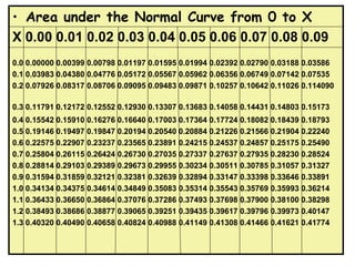
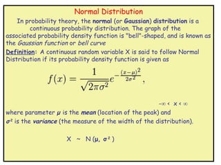
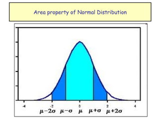
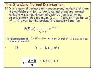
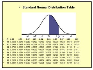
The normal distribution is a continuous probability distribution that is symmetric and bell-shaped. It is defined by two parameters: the mean (μ) and the standard deviation (σ). The standard normal distribution refers to a normal distribution with a mean of 0 and standard deviation of 1. The normal distribution and standard normal distribution have many useful properties and applications in statistics. Tables of the standard normal distribution are often used to find probabilities associated with the normal distribution.

1. NORMAL
DISTRIBUTION
(A Continuous Probability Distribution)

2. Normal Distribution
In probability theory, the normal (or Gaussian) distribution is a
continuous probability distribution. The graph of the
associated probability density function is "bell"-shaped, and is known as
the Gaussian function or bell curve
Definition: A continuous random variable X is said to follow Normal
Distribution if its probability density function is given as
-∞ < x < ∞
where parameter μ is the mean (location of the peak) and
σ 2 is the variance (the measure of the width of the distribution).
X ~ N (μ, σ 2 )

3. Area property of Normal Distribution

4. The Standard Normal Distribution:
If X is a normal variable with mean μ and variance σ 2 then
the variable z = (x- μ )/σ is called standard normal
variable A standard normal distribution is a normal
distribution with zero mean ( ) and unit variance (
), given by the probability density function
P(Z=z) =
The distribution of with μ = 0 and σ 2 = 1 is called the
standard normal.
• If X ~ N (μ, σ 2 )
~ N ( 0, 1 )

5. For normal variable infinite values of mean and variance
are possible that’s why it is to be standardize…

6. Properties of Normal Curve:
The normal curve with mean µ and standard deviation σ has following
properties
1. The equation of the curve is
2. The curve is symmetric about the line x = µ and x ranges from -∞ to
+∞.
3.Mean, mode and median coincide at x = µ as distribution is symmetrical.
4.The points of inflection of the curve are x = µ + σ and x = µ - σ.
5. In normal distribution Q.D.: M.D. : S.D. = 10 : 12 : 15
6.The M.D. about mean = 4/5 * S.D.
7.The normal curve has single peak i.e. unimodal.

7. 8.Area property of Normal Distribution

8. Area property of standard normal distribution

9. • Standard Normal Distribution Table
• Z 0.00 0.01 0.02 0.03 0.04 0.05 0.06 0.07 0.08 0.09
• 0.0 0.0000 0.0040 0.0080 0.0120 0.0160 0.0199 0.0239 0.0279 0.0319 0.0359
• 0.1 0.0398 0.0438 0.0478 0.0517 0.0557 0.0596 0.0636 0.0675 0.0714 0.0753
• 0.2 0.0793 0.0832 0.0871 0.0910 0.0948 0.0987 0.1026 0.1064 0.1103 0.1141
• 0.3 0.1179 0.1217 0.1255 0.1293 0.1331 0.1368 0.1406 0.1443 0.1480 0.1517
• 0.4 0.1554 0.1591 0.1628 0.1664 0.1700 0.1736 0.1772 0.1808 0.1844 0.1879
• 0.5 0.1915 0.1950 0.1985 0.2019 0.2054 0.2088 0.2123 0.2157 0.2190 0.2224
• 0.6 0.2257 0.2291 0.2324 0.2357 0.2389 0.2422 0.2454 0.2486 0.2517 0.2549
• 0.7 0.2580 0.2611 0.2642 0.2673 0.2704 0.2734 0.2764 0.2794 0.2823 0.2852
• 0.8 0.2881 0.2910 0.2939 0.2967 0.2995 0.3023 0.3051 0.3078 0.3106 0.3133

10. • Z 0.00 0.01 0.02 0.03 0.04 0.05 0.06 0.07 0.08 0.09
• 0.9 0.3159 0.3186 0.3212 0.3238 0.3264 0.3289 0.3315 0.3340 0.3365 0.3389
• 1.0 0.3413 0.3438 0.3461 0.3485 0.3508 0.3531 0.3554 0.3577 0.3599 0.3621
• 1.1 0.3643 0.3665 0.3686 0.3708 0.3729 0.3749 0.3770 0.3790 0.3810 0.3830
• 1.2 0.3849 0.3869 0.3888 0.3907 0.3925 0.3944 0.3962 0.3980 0.3997 0.4015
• 1.3 0.4032 0.4049 0.4066 0.4082 0.4099 0.4115 0.4131 0.4147 0.4162 0.4177
• 1.4 0.4192 0.4207 0.4222 0.4236 0.4251 0.4265 0.4279 0.4292 0.4306 0.4319
• 1.5 0.4332 0.4345 0.4357 0.4370 0.4382 0.4394 0.4406 0.4418 0.4429 0.4441
• 1.6 0.4452 0.4463 0.4474 0.4484 0.4495 0.4505 0.4515 0.4525 0.4535 0.4545
• 1.7 0.4554 0.4564 0.4573 0.4582 0.4591 0.4599 0.4608 0.4616 0.4625 0.4633
• 1.8 0.4641 0.4649 0.4656 0.4664 0.4671 0.4678 0.4686 0.4693 0.4699 0.4706
• 1.9 0.4713 0.4719 0.4726 0.4732 0.4738 0.4744 0.4750 0.4756 0.4761 0.4767
• 2.0 0.4772 0.4778 0.4783 0.4788 0.4793 0.4798 0.4803 0.4808 0.4812 0.4817
• 2.1 0.4821 0.4826 0.4830 0.4834 0.4838 0.4842 0.4846 0.4850 0.4854 0.4857
• 2.2 0.4861 0.4864 0.4868 0.4871 0.4875 0.4878 0.4881 0.4884 0.4887 0.4890
• 2.3 0.4893 0.4896 0.4898 0.4901 0.4904 0.4906 0.4909 0.4911 0.4913 0.4916
• 2.4 0.4918 0.4920 0.4922 0.4925 0.4927 0.4929 0.4931 0.4932 0.4934 0.4936
• 2.5 0.4938 0.4940 0.4941 0.4943 0.4945 0.4946 0.4948 0.4949 0.4951 0.4952
• 2.6 0.4953 0.4955 0.4956 0.4957 0.4959 0.4960 0.4961 0.4962 0.4963 0.4964
• 2.7 0.4965 0.4966 0.4967 0.4968 0.4969 0.4970 0.4971 0.4972 0.4973 0.4974
• 2.8 0.4974 0.4975 0.4976 0.4977 0.4977 0.4978 0.4979 0.4979 0.4980 0.4981
• 2.9 0.4981 0.4982 0.4982 0.4983 0.4984 0.4984 0.4985 0.4985 0.4986 0.4986
• 3.0 0.4987 0.4987 0.4987 0.4988 0.4988 0.4989 0.4989 0.4989 0.4990 0.4990
*************************

11. Normal Probability:
1] As normal distribution is continuous distribution,
probability at a point is zero i.e. P ( z = a ) = 0
2] As the standard normal distribution is symmetric about
mean (=0). P (z < 0 ) = P ( z > 0 ) = ½
3] P ( 0 < z < a) then table value for a gives the required
probability.
4] P (-a < z < 0) = P ( 0 < z < a) as the curve is symmetric
about 0.
5] P( z < -a) = P ( z > a) = P ( z > 0 ) - P ( 0 < z < a)

12. • 1]Question: What is the relative frequency of observations
below 1.18?
• That is, find the relative frequency of the event Z < 1.18. (Here
small z is 1.18.) (Or P(Z < 1.18 )
• P( z < 1.18) = P( z < 0 ) + P ( 0 < z < 1.18)
• = 0.5 + 0.3810
• = 0.8810

13. 2] P(z<-0.63) = P(z>0.63) = P(z>0) – P(0<z<063) = 0.2643
3] P(z>-1.48) = P(z>0) + P(0<z<1.48) = 0.9306

14. 4] P( -1.65 < z < 1.65 ) = 2 P ( 0< z < 1.65 )
5] P(z<0.84) = 0.8000

15. • Normal tables can be of this type P ( z < a )
• z. 00 .01.... 08. 09
• 0.0 .5000 .5040.... .5319 .5359
• 0.1 .5398 .5438.... .5714 .5753
• |
• |
• 1.0 .8413 .8438... .8599 .8621
• 1.1 .8643 .8665... .8810 .8830
• 1.2 .8849 .8869... .8997 .9015

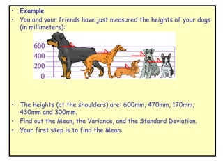
16. • Example 1
An average light bulb manufactured by the Acme
Corporation lasts 300 days with a standard deviation of
50 days. Assuming that bulb life is normally distributed,
what is the probability that an Acme light bulb will last
at most 365 days?
• Example 2
Suppose scores on an IQ test are normally distributed.
If the test has a mean of 100 and a standard deviation
of 10, what is the probability that a person who takes
the test will score between 90 and 110?
[P( 90 < X < 110 ) = P( X < 110 ) - P( X < 90 )
P( 90 < X < 110 ) = 0.84 - 0.16
P( 90 < X < 110 ) = 0.68
• Thus, about 68% of the test scores will fall between 90
and 110.]

17. • Problem 3
• Molly earned a score of 940 on a national achievement
test. The mean test score was 850 with a standard
deviation of 100. What proportion of students had a
higher score than Molly? (Assume that test scores are
normally distributed.)
• [z = (X - μ) / σ = (940 - 850) / 100 = 0.90
• we find P(Z < 0.90) = 0.8159.
Therefore, the P(Z > 0.90) = 1 - P(Z < 0.90) = 1 - 0.8159
= 0.1841. Thus, we estimate that 18.41 percent of the
students tested had a higher score than Molly. ]

18. 4.The Acme Light Bulb Company has found that an average light bulb
lasts 1000 hours with a standard deviation of 100 hours. Assume
that bulb life is normally distributed. What is the probability that
a randomly selected light bulb will burn out in 1200 hours or less?
5. Bill claims that he can do more push-ups than 90% of the boys in
his school. Last year, the average boy did 50 push-ups, with a
standard deviation of 10 pushups. Assume push-up performance is
normally distributed. How many pushups would Bill have to do to
beat 90% of the other boys?
***************

19. • Example
• You and your friends have just measured the heights of your dogs
(in millimeters):
• The heights (at the shoulders) are: 600mm, 470mm, 170mm,
430mm and 300mm.
• Find out the Mean, the Variance, and the Standard Deviation.
• Your first step is to find the Mean:

20. • Answer:
• Mean = [600 + 470 + 170 + 430 + 300]/5 = 1970/5 = 394
•
• so the mean (average) height is 394 mm. Let's plot this on the
chart:
• Now, we calculate each dogs difference from the Mean:

21. • To calculate the Variance, take each difference, square it, and then average the
result:
• Variance: σ2 = [2062 + 762 + (-224)2 + 362 + (-94)2 ]/5 = 108,520/5 = 21,704
• So, the Variance is 21,704.
• And the Standard Deviation is just the square root of Variance, so:
• Standard Deviation: σ = √21,704 = 147.32... = 147 (to the nearest mm)
•
• And the good thing about the Standard Deviation is that it is useful. Now we can
show which heights are within one Standard Deviation (147mm) of the Mean:
• So, using the Standard Deviation we have a "standard" way of knowing what is
normal, and what is extra large or extra small.

22. • Area under the Normal Curve from 0 to X
X 0.00 0.01 0.02 0.03 0.04 0.05 0.06 0.07 0.08 0.09
0.0 0.00000 0.00399 0.00798 0.01197 0.01595 0.01994 0.02392 0.02790 0.03188 0.03586
0.1 0.03983 0.04380 0.04776 0.05172 0.05567 0.05962 0.06356 0.06749 0.07142 0.07535
0.2 0.07926 0.08317 0.08706 0.09095 0.09483 0.09871 0.10257 0.10642 0.11026 0.114090
0.3 0.11791 0.12172 0.12552 0.12930 0.13307 0.13683 0.14058 0.14431 0.14803 0.15173
0.4 0.15542 0.15910 0.16276 0.16640 0.17003 0.17364 0.17724 0.18082 0.18439 0.18793
0.5 0.19146 0.19497 0.19847 0.20194 0.20540 0.20884 0.21226 0.21566 0.21904 0.22240
0.6 0.22575 0.22907 0.23237 0.23565 0.23891 0.24215 0.24537 0.24857 0.25175 0.25490
0.7 0.25804 0.26115 0.26424 0.26730 0.27035 0.27337 0.27637 0.27935 0.28230 0.28524
0.8 0.28814 0.29103 0.29389 0.29673 0.29955 0.30234 0.30511 0.30785 0.31057 0.31327
0.9 0.31594 0.31859 0.32121 0.32381 0.32639 0.32894 0.33147 0.33398 0.33646 0.33891
1.0 0.34134 0.34375 0.34614 0.34849 0.35083 0.35314 0.35543 0.35769 0.35993 0.36214
1.1 0.36433 0.36650 0.36864 0.37076 0.37286 0.37493 0.37698 0.37900 0.38100 0.38298
1.2 0.38493 0.38686 0.38877 0.39065 0.39251 0.39435 0.39617 0.39796 0.39973 0.40147
1.3 0.40320 0.40490 0.40658 0.40824 0.40988 0.41149 0.41308 0.41466 0.41621 0.41774