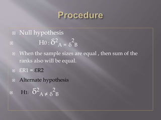
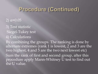
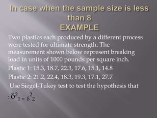
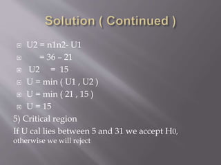
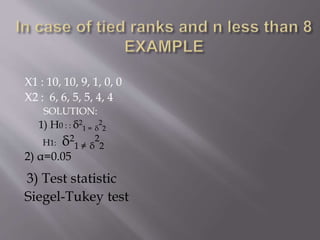
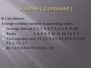
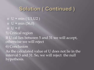
 Siegel-Tukey test named after Sidney Siegel and
John Tukey, is a non-parametric test which may be
applied to the data measured at least on an ordinal
scale. It tests for the differences in scale between
two groups.
 The test is used to determine if one of two groups
of data tends to have more widely dispersed
values than the other.
 The test was published in 1980 by Sidney Siegel
and John Wilder Tukey in the journal of the
American Statistical Association in the article “A
Non-parametric Sum Of Ranks Procedure For
Relative Spread in Unpaired Samples “.
 Each sample has been randomly selected from
the population.
 The two samples are independent of one
another.
 The level of measurement the data represent is
at least ordinal.
 The two populations from which the samples
are derived have equal medians.
 Null hypothesis
 H0 : δ2
A = δ
2
B
 When the sample sizes are equal , then sum of the
ranks also will be equal.
 ԐR1 = ԐR2
 Alternate hypothesis
 H1: δ2
A ≠ δ
2
B
2) α=0.05
3) Test statistic
Siegel-Tukey test
4) Calculations
By combining the groups. The ranking is done by
alternate extremes (rank 1 is lowest, 2 and 3 are the
two highest, 4 and 5 are the two next lowest etc)
Sum the rank of first and second group, after this
procedure apply Mann-Whitney U test to find out
the U value.
 U1 = n1n2+n1(n1+1)/2‒ ԐR1
 U2 = n1n2+n2(n2+1)‒ԐR2
 U = Min( U1,U2)
5)Critical region
Ucal ˂ Utab ˂ Ucal
6) Conclusion
Accept or reject H0
Two plastics each produced by a different process
were tested for ultimate strength. The
measurement shown below represent breaking
load in units of 1000 pounds per square inch.
Plastic 1: 15.3, 18.7, 22.3, 17.6, 15.1, 14.8
Plastic 2: 21.2, 22.4, 18.3, 19.3, 17.1, 27.7
Use Siegel-Tukey test to test the hypothesis that
: δ2
1 = δ
2
2
1) H0 : : δ2
1 = δ
2
2
H1: δ2
1 ≠ δ
2
2
2) α=0.05
3) Test statistic
Siegel-Tukey test
4) Calculations
Arrange combine samples in ascending
order,
 14.8, 15.1, 15.3, 17.1, 17.6, 18.3, 18.7, 19.3,
 1 4 5 8 9 12 11 10
 21.2, 22.3, 22.4, 27.7
 7 6 3 2
 R1 = 1+4+5+9+11+6 = 36
 R2 = 8+12+10+7+3+2 = 42
 U1 = n1n2+n1(n1+1)/2‒ ԐR1
 = 36+6( 6+1 ) /2 – 36
 =21
 U2 = n1n2- U1
 = 36 – 21
 U2 = 15
 U = min ( U1 , U2 )
 U = min ( 21 , 15 )
 U = 15
5) Critical region
If U cal lies between 5 and 31 we accept H0,
otherwise we will reject
6) Conclusion
As the calculated value of U lies in the interval 5
and 31. So, we accept the null hypothesis.
X1 : 10, 10, 9, 1, 0, 0
X2 : 6, 6, 5, 5, 4, 4
SOLUTION:
1) H0 : : δ2
1 = δ
2
2
H1: δ2
1 ≠ δ
2
2
2) α=0.05
3) Test statistic
Siegel-Tukey test
4) Calculations
Arrange combine samples in ascending order,
 Arrange data set 0, 0, 1, 4, 4, 5, 5, 6, 6, 9, 10, 10
 Ranks 1 4 5 8 9 12 11 10 7 6 3 2
 Tied adjusted rank 2.5, 2.5, 5, 8.5, 8.5, 11.5, 11.5, 8.5,
8.5, 6, 2.5, 2.5
 R1 = 2.5+2.5+6+5+2.5+2.5 = 21
 R2 = 8.5 +8.5+11.5+11.5+8.5+8.5 = 57
 U1 = n1n2+n1(n1+1)/2‒ ԐR1
 U1 = 36+6( 6+1)/2 – 21
 U1 = 36+21 – 21
 U1 = 36
 U2 = n1n2 – U1
 U2 = 36 – 36
 U2 = 0
 U = min ( U1,U2 )
 U = min (36,0)
 U = 0
5) Critical region
If U cal lies between 5 and 31 we will accept,
otherwise we will reject
6) Conclusion
As the calculated value of U does not lie in the
interval 5 and 31. So, we will reject the null
hypothesis.
If the sample size is greater than 8 and there are tied
ranks in the data. We will use the formula
𝑧 =
𝑢−𝑛1𝑛2
2
𝑛1𝑛2 𝑛1+𝑛2+1
12
−
𝑛1𝑛2 Σs 𝑡3−𝑡
12𝑛1𝑛2 𝑛1+𝑛2−1
Where s denotes the no of pair of ties
and t denotes no of tied ranks
 Group 1: 3.1, 5.3, 6.4, 6.2, 3.8, 7.5, 5.8, 4.3, 5.9, 4.9
 Group 2: 9, 5.6, 6.3, 8.5, 4.6, 7.1, 5.5, 7.9, 6.8, 5.7,
8.9
Solution:
1) H0 : : δ2
1 = δ
2
2
H1: δ2
1 ≠ δ
2
2
2) α=0.05
3) Test statistic
Siegel-Tukey test
4) Calculations
Arrange combine samples in ascending order
 3.1, 3.8, 4.3, 4.6, 4.9, 5.3, 5.5, 5.6, 5.7, 5.8,
 1 4 5 8 9 12 13 16 17 20
 5.9, 6.2, 6.3, 6.4, 6,8, 7.1, 7.5, 7.9, 8.5, 8.9, 9.0
 21 19 18 15 14 11 10 7 6 3 2
R1 = 1+4+5+9+12+20+21+19+15+10 = 116
R2 = 8+13+16+17+18+14+11+7+6+3+2 = 115
U1 = n1n2+n1(n1+1)/2‒ ԐR1
U1 = 10(11)+10(10+1)/2 – 116
U1 = 149
U2 = n1n2+n2(n2+1)‒ԐR2
U2 = 10(11)+11(11+1)/2 – 115
U2 = 61
 U=min( U1,U2 )
 U=min( 149,61 )
 U=61
 𝑧 =
𝑢−
𝑛1𝑛2
2
𝑛1𝑛2 𝑛1+𝑛2+1
12
 𝑧 =
61−
10(11)
2
10(11) 10+11+1
12
 Z = 0.42
5) Critical region
If Zcal ≥ Ztab we reject our null hypothesis
6) Conclusion
Since calculated value is less than tabulated value. So,
we accept the null hypothesis.
THANK
YOU

The siegel-tukey-test-for-equal-variability

  • 1.
     Siegel-Tukey testnamed after Sidney Siegel and John Tukey, is a non-parametric test which may be applied to the data measured at least on an ordinal scale. It tests for the differences in scale between two groups.  The test is used to determine if one of two groups of data tends to have more widely dispersed values than the other.  The test was published in 1980 by Sidney Siegel and John Wilder Tukey in the journal of the American Statistical Association in the article “A Non-parametric Sum Of Ranks Procedure For Relative Spread in Unpaired Samples “.
  • 2.
     Each samplehas been randomly selected from the population.  The two samples are independent of one another.  The level of measurement the data represent is at least ordinal.  The two populations from which the samples are derived have equal medians.
  • 3.
     Null hypothesis H0 : δ2 A = δ 2 B  When the sample sizes are equal , then sum of the ranks also will be equal.  ԐR1 = ԐR2  Alternate hypothesis  H1: δ2 A ≠ δ 2 B
  • 4.
    2) α=0.05 3) Teststatistic Siegel-Tukey test 4) Calculations By combining the groups. The ranking is done by alternate extremes (rank 1 is lowest, 2 and 3 are the two highest, 4 and 5 are the two next lowest etc) Sum the rank of first and second group, after this procedure apply Mann-Whitney U test to find out the U value.
  • 5.
     U1 =n1n2+n1(n1+1)/2‒ ԐR1  U2 = n1n2+n2(n2+1)‒ԐR2  U = Min( U1,U2) 5)Critical region Ucal ˂ Utab ˂ Ucal 6) Conclusion Accept or reject H0
  • 6.
    Two plastics eachproduced by a different process were tested for ultimate strength. The measurement shown below represent breaking load in units of 1000 pounds per square inch. Plastic 1: 15.3, 18.7, 22.3, 17.6, 15.1, 14.8 Plastic 2: 21.2, 22.4, 18.3, 19.3, 17.1, 27.7 Use Siegel-Tukey test to test the hypothesis that : δ2 1 = δ 2 2
  • 7.
    1) H0 :: δ2 1 = δ 2 2 H1: δ2 1 ≠ δ 2 2 2) α=0.05 3) Test statistic Siegel-Tukey test 4) Calculations Arrange combine samples in ascending order,
  • 8.
     14.8, 15.1,15.3, 17.1, 17.6, 18.3, 18.7, 19.3,  1 4 5 8 9 12 11 10  21.2, 22.3, 22.4, 27.7  7 6 3 2  R1 = 1+4+5+9+11+6 = 36  R2 = 8+12+10+7+3+2 = 42  U1 = n1n2+n1(n1+1)/2‒ ԐR1  = 36+6( 6+1 ) /2 – 36  =21
  • 9.
     U2 =n1n2- U1  = 36 – 21  U2 = 15  U = min ( U1 , U2 )  U = min ( 21 , 15 )  U = 15 5) Critical region If U cal lies between 5 and 31 we accept H0, otherwise we will reject
  • 10.
    6) Conclusion As thecalculated value of U lies in the interval 5 and 31. So, we accept the null hypothesis.
  • 11.
    X1 : 10,10, 9, 1, 0, 0 X2 : 6, 6, 5, 5, 4, 4 SOLUTION: 1) H0 : : δ2 1 = δ 2 2 H1: δ2 1 ≠ δ 2 2 2) α=0.05 3) Test statistic Siegel-Tukey test
  • 12.
    4) Calculations Arrange combinesamples in ascending order,  Arrange data set 0, 0, 1, 4, 4, 5, 5, 6, 6, 9, 10, 10  Ranks 1 4 5 8 9 12 11 10 7 6 3 2  Tied adjusted rank 2.5, 2.5, 5, 8.5, 8.5, 11.5, 11.5, 8.5, 8.5, 6, 2.5, 2.5  R1 = 2.5+2.5+6+5+2.5+2.5 = 21
  • 13.
     R2 =8.5 +8.5+11.5+11.5+8.5+8.5 = 57  U1 = n1n2+n1(n1+1)/2‒ ԐR1  U1 = 36+6( 6+1)/2 – 21  U1 = 36+21 – 21  U1 = 36  U2 = n1n2 – U1  U2 = 36 – 36  U2 = 0
  • 14.
     U =min ( U1,U2 )  U = min (36,0)  U = 0 5) Critical region If U cal lies between 5 and 31 we will accept, otherwise we will reject 6) Conclusion As the calculated value of U does not lie in the interval 5 and 31. So, we will reject the null hypothesis.
  • 15.
    If the samplesize is greater than 8 and there are tied ranks in the data. We will use the formula 𝑧 = 𝑢−𝑛1𝑛2 2 𝑛1𝑛2 𝑛1+𝑛2+1 12 − 𝑛1𝑛2 Σs 𝑡3−𝑡 12𝑛1𝑛2 𝑛1+𝑛2−1 Where s denotes the no of pair of ties and t denotes no of tied ranks
  • 16.
     Group 1:3.1, 5.3, 6.4, 6.2, 3.8, 7.5, 5.8, 4.3, 5.9, 4.9  Group 2: 9, 5.6, 6.3, 8.5, 4.6, 7.1, 5.5, 7.9, 6.8, 5.7, 8.9 Solution: 1) H0 : : δ2 1 = δ 2 2 H1: δ2 1 ≠ δ 2 2 2) α=0.05 3) Test statistic Siegel-Tukey test
  • 17.
    4) Calculations Arrange combinesamples in ascending order  3.1, 3.8, 4.3, 4.6, 4.9, 5.3, 5.5, 5.6, 5.7, 5.8,  1 4 5 8 9 12 13 16 17 20  5.9, 6.2, 6.3, 6.4, 6,8, 7.1, 7.5, 7.9, 8.5, 8.9, 9.0  21 19 18 15 14 11 10 7 6 3 2 R1 = 1+4+5+9+12+20+21+19+15+10 = 116
  • 18.
    R2 = 8+13+16+17+18+14+11+7+6+3+2= 115 U1 = n1n2+n1(n1+1)/2‒ ԐR1 U1 = 10(11)+10(10+1)/2 – 116 U1 = 149 U2 = n1n2+n2(n2+1)‒ԐR2 U2 = 10(11)+11(11+1)/2 – 115 U2 = 61
  • 19.
     U=min( U1,U2)  U=min( 149,61 )  U=61  𝑧 = 𝑢− 𝑛1𝑛2 2 𝑛1𝑛2 𝑛1+𝑛2+1 12  𝑧 = 61− 10(11) 2 10(11) 10+11+1 12
  • 20.
     Z =0.42 5) Critical region If Zcal ≥ Ztab we reject our null hypothesis 6) Conclusion Since calculated value is less than tabulated value. So, we accept the null hypothesis.
  • 21.