This document provides an introduction to the normal distribution and the standard normal distribution. It includes:
- Information on the key characteristics of the normal distribution and how it is defined by the mean and standard deviation.
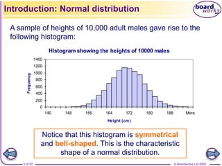
- Examples of real-world data that can be modeled by the normal distribution.
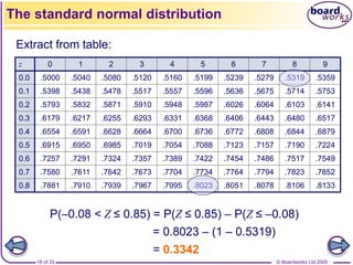
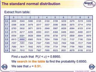
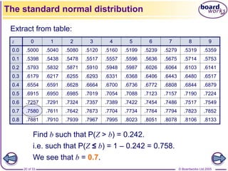
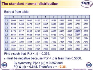
- An explanation of the standard normal distribution and how probability tables are used to find probabilities for this distribution.
- Worked examples of calculating probabilities using the standard normal distribution tables.


![© Boardworks Ltd 2005
6 of 33
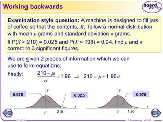
If X has a normal distribution with mean μ, and variance σ2,
we write
X ~ N[μ, σ2]
68% of the distribution lies within
1 standard deviation of the mean.
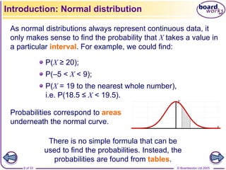
Introduction: Normal distribution
x
y
μ – σ μ + σ](https://image.slidesharecdn.com/normal-distribution-2-230510011130-1707a444/85/normal-distribution-2-ppt-6-320.jpg)
![© Boardworks Ltd 2005
7 of 33
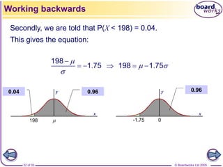
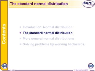
95% of the distribution lies within 2
standard deviations of the mean.
Introduction: Normal distribution
x
y
If X has a normal distribution with mean μ, and variance σ2,
we write
X ~ N[μ, σ2]
μ – 2σ μ + 2σ](https://image.slidesharecdn.com/normal-distribution-2-230510011130-1707a444/85/normal-distribution-2-ppt-7-320.jpg)
![© Boardworks Ltd 2005
8 of 33
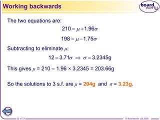
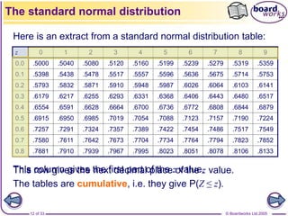
99.7% of the distribution lies within
3 standard deviations of the mean.
Introduction: Normal distribution
x
y
If X has a normal distribution with mean μ, and variance σ2,
we write
X ~ N[μ, σ2]
μ + 3σ
μ – 3σ](https://image.slidesharecdn.com/normal-distribution-2-230510011130-1707a444/85/normal-distribution-2-ppt-8-320.jpg)
![© Boardworks Ltd 2005
11 of 33
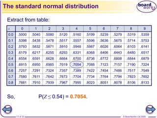
The normal distribution with mean 0 and standard deviation 1
is called the standard normal distribution – it is denoted Z.
So, Z ~ N[0, 1].
Probabilities for this distribution are given in tables.
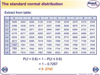
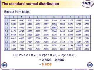
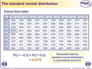
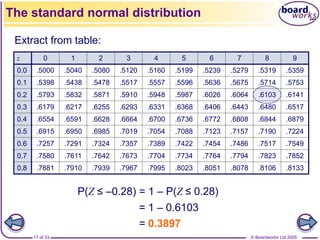
The standard normal distribution
-3 -2 -1 1 2 3
x
y](https://image.slidesharecdn.com/normal-distribution-2-230510011130-1707a444/85/normal-distribution-2-ppt-11-320.jpg)
![© Boardworks Ltd 2005
23 of 33
It would of course be impractical to publish tables of
probabilities for every possible normal distribution.
Fortunately, it is possible and easy to transform any
normal distribution to a standard normal:
If X ~ then ~ [ ].
N 0,1
X
Z
[ , ]
2
N
Standardise
[ ]
N 0, 1
More general normal distributions
x
y
[ , ]
2
N
-3 -2 -1 1 2 3
x
y](https://image.slidesharecdn.com/normal-distribution-2-230510011130-1707a444/85/normal-distribution-2-ppt-23-320.jpg)
![© Boardworks Ltd 2005
24 of 33
Example: If , find
a) P(X < 23);
b) P(X > 14);
c) P(16 < X < 24.8).
~ [ , ]
N 20 16
X
a) If σ2 = 16, then σ = 4.
( ) ( . )
P 23 P 0 75
X Z
More general normal distributions
x
y
x
y
20 23 0 0.75
Standardise
.
23 20
0 75
4
= 0.7734](https://image.slidesharecdn.com/normal-distribution-2-230510011130-1707a444/85/normal-distribution-2-ppt-24-320.jpg)
![© Boardworks Ltd 2005
25 of 33
b)
( ) ( . ) ( . )
P 14 P 1 5 P 1 5
X Z Z
More general normal distributions
Example: If , find
a) P(X < 23);
b) P(X > 14);
c) P(16 < X < 24.8).
~ [ , ]
N 20 16
X
x
y
x
y
14 20 –1.5 0
Standardise
.
14 20
1 5
4
= 0.9332](https://image.slidesharecdn.com/normal-distribution-2-230510011130-1707a444/85/normal-distribution-2-ppt-25-320.jpg)
![© Boardworks Ltd 2005
26 of 33
c)
.
. ( . )
16 20 24 8 20
P 16 24 8 P P 1 1 2
4 4
X Z Z
P(Z < 1.2) = 0.8849
and P(Z < –1) = 1 – P(Z < 1) = 1 – 0.8413 = 0.1587.
So, P(–1 < Z < 1.2) = 0.8849 – 0.1587 = 0.7262
More general normal distributions
Example: If , find
a) P(X < 23);
b) P(X > 14);
c) P(16 < X < 24.8).
~ [ , ]
N 20 16
X
x
y
x
y
Standardise
16 20 24.8 -1 0 1.2](https://image.slidesharecdn.com/normal-distribution-2-230510011130-1707a444/85/normal-distribution-2-ppt-26-320.jpg)
![© Boardworks Ltd 2005
27 of 33
Let X be the random variable for the IQ of an individual.
X ~ N[100, 225].
So, we want P(X > 124) = P(Z > 1.6)
= 1 – P(Z ≤ 1.6) = 1 – 0.9452
More general normal distributions
Examination style question: IQs are normally distributed
with mean 100 and standard deviation 15. What proportion
of the population have an IQ of at least 124?
x
y
x
y
100 124 0 1.6
Standardise
.
124 100
1 6
15
= 0.0548](https://image.slidesharecdn.com/normal-distribution-2-230510011130-1707a444/85/normal-distribution-2-ppt-27-320.jpg)
![© Boardworks Ltd 2005
29 of 33
x
y
To find x, we start by finding the standardised value z such
that P(Z < z) = 0.67.
From tables we see that z = 0.44.
We therefore need to find the value that standardises to
make 0.44 by rearranging the formula.
Example: If X ~ N[4, 0.25], find the value of
x if P(X < x) = 0.67.
Working backwards
x
y
4 x 0 0.44
Standardise
[ . ]
N 4, 0 25 [ ]
N 0, 1
.
.
.
4 0 44 0
4 22
5
x
x
](https://image.slidesharecdn.com/normal-distribution-2-230510011130-1707a444/85/normal-distribution-2-ppt-29-320.jpg)
![© Boardworks Ltd 2005
30 of 33
x
y
x
y
Let X represent the marks in the examination. X ~ N[62, 256].
We need to find x such that P(X ≥ x) = 0.86.
We need to solve: . Therefore x = 44.72.
Example: Marks in an examination can be assumed to
follow a normal distribution with mean 62 and standard
deviation 16. The pass mark is to be chosen so that 86%
of candidates pass. Find the pass mark.
-1.08
.
62
1 08
16
x
x
Working backwards
Standardise
So, the pass mark is 44.](https://image.slidesharecdn.com/normal-distribution-2-230510011130-1707a444/85/normal-distribution-2-ppt-30-320.jpg)