Download as PDF, PPTX

![Ito Isometry
Let Xt : [0, T] × Ω → R be a stochastic process adapted to filtration
F of brownian motion zt.
Then, we know that the Ito integral
T
0 Xt · dzt is a martingale
Ito Isometry tells us about the variance of
T
0 Xt · dzt
E[(
T
0
Xt · dzt)2
] = E[
T
0
X2
t · dt]
Extending this to two Ito integrals, we have:
E[(
T
0
Xt · dzt)(
T
0
Yt · dzt)] = E[
T
0
Xt · Yt · dt]
Ashwin Rao (Stanford) Stochastic Calculus Foundations November 13, 2018 5 / 11](https://image.slidesharecdn.com/stochasticcalculusfoundations-181114014957/75/Overview-of-Stochastic-Calculus-Foundations-5-2048.jpg)
![Feynman-Kac Formula (PDE-SDE linkage)
Consider the partial differential equation for u : R × [0, T] → R:
∂u(x, t)
∂t
+µ(x, t)
∂u(x, t)
∂x
+
σ2(x, t)
2
∂2u(x, t)
∂x2
−V (x, t)u(x, t) = f (x, t)
subject to u(x, T) = ψ(x), where µ, σ, V , f , ψ are known functions.
Then the Feynman-Kac formula tells us that the solution u(x, t) can
be written as the following conditional expectation:
E[(
T
t
e− u
t V (Xs ,s)ds
· f (Xu, u) · du) + e− T
t V (Xu,u)du
· ψ(XT )|Xt = x]
such that Xu is the following Ito process with initial condition Xt = x:
dXu = µ(Xu, u) · du + σ(Xu, u) · dzu
Ashwin Rao (Stanford) Stochastic Calculus Foundations November 13, 2018 7 / 11](https://image.slidesharecdn.com/stochasticcalculusfoundations-181114014957/75/Overview-of-Stochastic-Calculus-Foundations-7-2048.jpg)
![Stopping Time
Stopping time τ is a “random time” (random variable) interpreted as
time at which a given stochastic process exhibits certain behavior
Stopping time often defined by a “stopping policy” to decide whether
to continue/stop a process based on present position and past events
Random variable τ such that Pr[τ ≤ t] is in σ-algebra Ft, for all t
Deciding whether τ ≤ t only depends on information up to time t
Hitting time of a Borel set A for a process Xt is the first time Xt
takes a value within the set A
Hitting time is an example of stopping time. Formally,
TX,A = min{t ∈ R|Xt ∈ A}
eg: Hitting time of a process to exceed a certain fixed level
Ashwin Rao (Stanford) Stochastic Calculus Foundations November 13, 2018 8 / 11](https://image.slidesharecdn.com/stochasticcalculusfoundations-181114014957/75/Overview-of-Stochastic-Calculus-Foundations-8-2048.jpg)
![Optimal Stopping Problem
Optimal Stopping problem for Stochastic Process Xt:
V (x) = max
τ
E[G(Xτ )|X0 = x]
where τ is a set of stopping times of Xt, V (·) is called the value
function, and G is called the reward (or gain) function.
Note that sometimes we can have several stopping times that
maximize E[G(Xτ )] and we say that the optimal stopping time is the
smallest stopping time achieving the maximum value.
Example of Optimal Stopping: Optimal Exercise of American Options
Xt is stochastic process for underlying security’s price
x is underlying security’s current price
τ is set of exercise times corresponding to various stopping policies
V (·) is American option price as function of underlying’s current price
G(·) is the option payoff function
Ashwin Rao (Stanford) Stochastic Calculus Foundations November 13, 2018 9 / 11](https://image.slidesharecdn.com/stochasticcalculusfoundations-181114014957/75/Overview-of-Stochastic-Calculus-Foundations-9-2048.jpg)
![Infinitesimal Generator and Dynkin’s Formula
Infinitesimal Generator of a time-homogeneous Rn-valued diffusion Xt
is the PDE operator A (operating on functions f : Rn → R) defined as
A • f (x) = lim
t→0
E[f (Xt)|X0 = x] − f (x)
t
For Rn-valued diffusion Xt given by: dXt = µ(Xt) · dt + σ(Xt) · dzt,
A • f (x) =
i
µi (x)
∂f
∂xi
(x) +
i,j
(σ(x)σ(x)T
)i,j
∂2f
∂xi ∂xj
(x)
If τ is stopping time conditional on X0 = x, Dynkin’s formula says:
E[f (Xτ )|X0 = x] = f (x) + E[
τ
0
A • f (Xs) · ds|X0 = x]
Stochastic generalization of 2nd fundamental theorem of calculus
Ashwin Rao (Stanford) Stochastic Calculus Foundations November 13, 2018 11 / 11](https://image.slidesharecdn.com/stochasticcalculusfoundations-181114014957/75/Overview-of-Stochastic-Calculus-Foundations-11-2048.jpg)

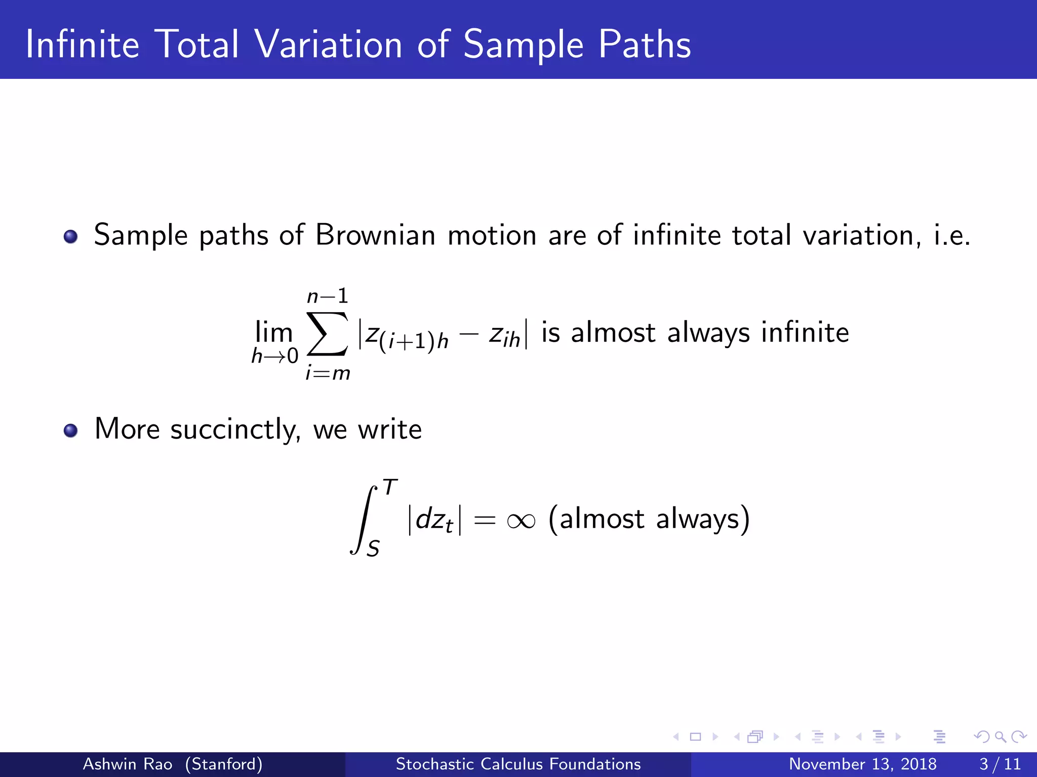
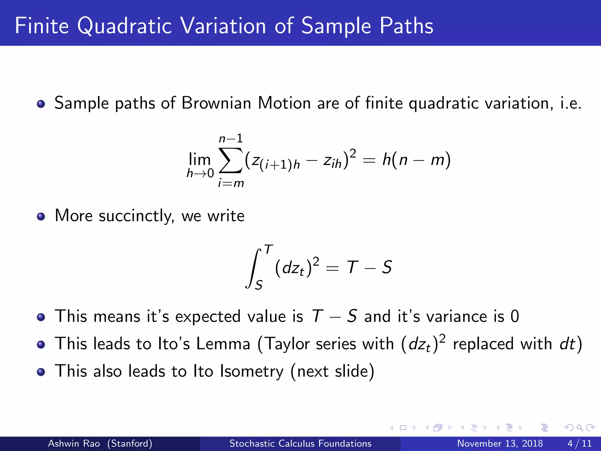
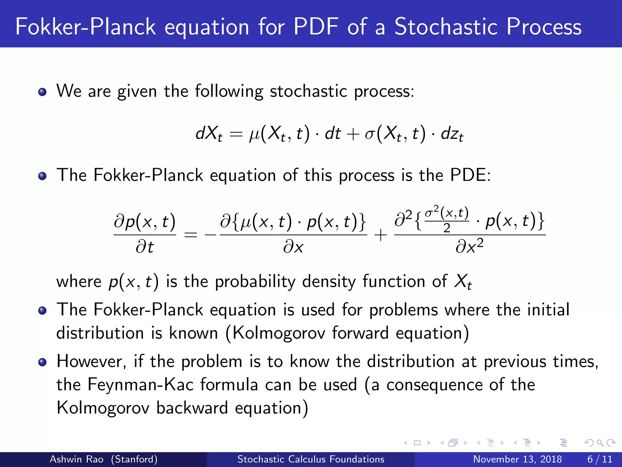
1) Sample paths of Brownian motion are continuous but almost always non-differentiable. They are of infinite total variation but finite quadratic variation. 2) Ito's lemma and Ito isometry relate stochastic integrals of Brownian motion to integrals of deterministic functions, allowing stochastic processes to be analyzed using tools from calculus and probability theory. 3) The Fokker-Planck and Kolmogorov equations link stochastic differential equations to partial differential equations governing the probability density function of the process, while the Feynman-Kac formula relates certain PDEs to conditional expectations of the process.