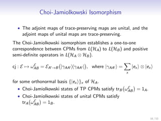
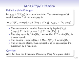
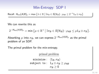
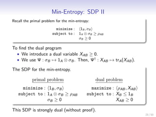
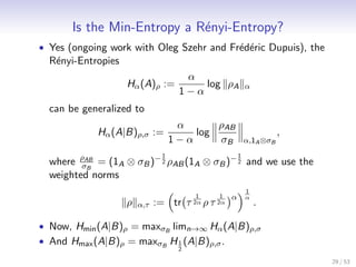
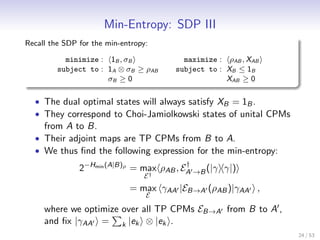
Let me summarize the key points: - The min-entropy of a state ρAB can be expressed as the optimal value of a semi-definite program (SDP) - The SDP has a primal and dual problem - Solving the dual problem gives an operator XAB that achieves the max of the dual objective ρAB, XAB - The optimal dual states satisfy XB = 1B and correspond to Choi-Jamiolkowski states of unital CPMs - This formulation allows the min-entropy to be computed by solving an SDP, which can be done efficiently for small systems

1. Smooth Entropies — A Tutorial
With Focus on Applications in Cryptography.
Marco Tomamichel
CQT, National University of Singapore
Singapore, September 14, 2011
1 / 53

2. Outline
1. Short Motivation and Overview of Applications
2. Preliminaries
3. Definition of the Min-Entropy and Smoothing
4. Some Useful Properties
• Data-Processing
• The Asymptotic Equipartition Property
• An Entropic Uncertainty Relation
5. Example Application: Proving Security of Quantum Key
Distribution on four slides.
Remember:
My goal: After this tutorial, you feel comfortable with the
min-entropy and understand how it is applied.
Please interrupt and ask questions at any time!
2 / 53

3. Motivation and Overview
Just a quick overview.
3 / 53

4. Entropic Approach to Information I
• Probability theory offers many advantages to describe
cryptographic problems.
• For example, how do we describe a secret key?
X = ”01010100100111001110100”
Is this string secret? From whom? We cannot tell unless we
know how it is created.
• Instead, we look at the joint probability distribution over
potential strings and side information, PXE . Here, E is any
information a potential adversary might hold about X .
• If PX is uniform and independent of E , we call it secret.
4 / 53

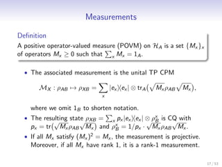
5. Entropic Approach to Information II
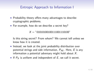
• We can also describe this situation with entropy [Sha48].
• Shannon defined the surprisal of an event X = x as
S(x)P = − log P(x).
• We can thus call a string secret if the average surprisal,
H(X )P = x P(x)S(x)P , is large.
• Entropies are measures of uncertainty about (the value of) a
random variable.
• There are other entropies, for example the min-entropy or
R´nyi entropy [R´n61] of order ∞.
e e
Hmin (X ) = min S(x)P .
x
• The min-entropy quantifies how hard it is to guess X . (The
optimal guessing strategy is to guess the most likely event,
and the probability of success is pguess (X )P = 2−Hmin (X )P .)
5 / 53

6. Entropic Approach to Information III
• Entropies can be easily extended to (classical) side
information, using conditional probability distributions.
• In the quantum setting, conditional states are not available
(there exist some definitions, but none of them appear very
useful) and the entropic approach is often the only available
option to quantify information.
• The von Neumann entropy generalizes Shannon’s entropy to
the quantum setting,
H(A|B)ρ := H(ρAB ) − H(ρB ), H(ρ) = −tr(ρ log ρ).
• This tutorial is concerned with a quantum extension of the
min-entropy.
6 / 53

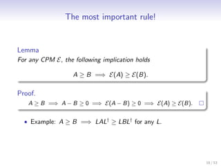
7. Foundations
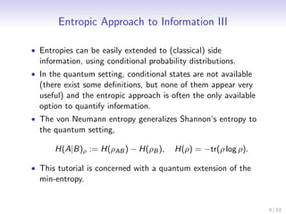
• The quantum generalization of the conditional min- and
max-entropy was introduced by Renner [Ren05] in his thesis.
• The main purpose was to generalize a theorem on privacy
amplification to the quantum setting.
• Since then, the smooth entropy framework has been
consolidated and extended [Tom12].
• The definition of Hmax is not what it used to be [KRS09].
• The smoothing is now done with regards to the purified
distance [TCR10].
• A relative entropy based on the quantum generalization of the
min-entropy was introduced by Datta [Dat09].
7 / 53

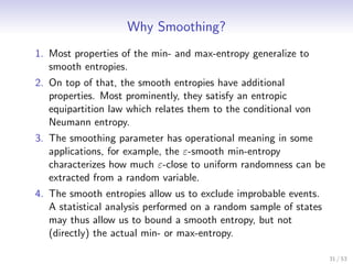
8. Applications
Smooth Min- and Max-Entropies have many applications.
Cryptography: Privacy Amplification [RK05, Ren05], Quantum
Key Distribution [Ren05, TLGR12], Bounded Storage
Model [DrFSS08, WW08] and Noisy Storage
Model [KWW12], No Go for Bit Commitment
[WTHR11] and OT [WW12] growing.
Information Theory: One-Shot Characterizations of Operational
Quantities (e.g. [Ber08], [BD10]).
Thermodynamics: One-Shot Work Extraction [DRRV11] and
Erasure [dRAR+ 11].
Uncertainty: Entropic Uncertainty Relations with Quantum Side
Information [BCC+ 10, TR11].
Correlations: To Investigate Correlations, Entanglement and
Decoupling (e.g. [Dup09, DBWR10, Col12]).
8 / 53

9. Mathematical Preliminaries
Stay with me through this part, after which I hope everybody is on
the same level.
9 / 53

10. Hilbert Spaces and Operators
Definition
A finite-dimensional Hilbert space, denoted H, is a vector space
with an inner product, · , · .
• Elements of H are written as kets, e.g. |ψ ∈ H.
• The set of linear operators from H to H is denoted L(H, H ).
• Adjoint operators L† to L are (uniquely) defined via the
relation |ψ , L|φ = L† |ψ , |φ .
• To simplify notation, we just write such an inner product as
ψ|L|φ = |ψ , L|φ .
• L(H, H ) is a Hilbert space with the Hilbert-Schmidt inner
product L, K = tr(L† K ).
10 / 53

11. Positive Operators
• We use L(H) := L(H, H) for operators mapping H onto itself.
• An operator L ∈ L(H) is called Hermitian (or self-adjoint) if it
satisfies L = L† .
Definition
A linear operator A ∈ L(H) is called positive semi-definite if
A = A† and ∀ |ψ ∈ H : ψ|A|ψ ≥ 0.
• We write A ≥ B if A − B is positive semi-definite.
√
• Operators |L| := L† L are always positive semi-definite.
• The operator 1 is the identity operator on H.
11 / 53

12. Tensor Spaces
• We distinguish mathematical objects corresponding to
different physical systems using subscripts.
• The tensor product space HA ⊗ HB is a vector space of linear
combinations of elements |ψA ⊗ |ψB , modulus
α |ψA ⊗ |ψB ≡ (α|ψA ) ⊗ |ψB ≡ |ψA ⊗ (α|ψB ) ,
|ψA ⊗ |ψB + |ψA ⊗ |φB ≡ |ψA ⊗ |ψB + |φB and
|ψA ⊗ |ψB + |φA ⊗ |ψB ≡ |ψA + |φA ⊗ |ψB ,
where |ψA , |φA ∈ HA and |ψB , |φB ∈ HB .
• Its inner product is a sesquilinear extension of
|ψA ⊗ |ψB , |φA ⊗ |φB = ψA |φA ψB |φB .
12 / 53

13. Quantum States
Definition
A quantum state is an operator ρA ≥ 0 with tr(ρA ) = 1.
• The set of quantum states on a Hilbert space HA is S(HA ).
• We say a quantum state ρXB ∈ HX ⊗ HB is classical-quantum
(CQ) if it is of the form
ρXB = px |ex ex | ⊗ ρx ,
B
x
where {px }x is a probability distribution, {|ex }x a fixed
orthonormal basis of HX , and ρx ∈ S(HB ).
B
• A state is pure if it has rank 1, i.e., if it can be written as
ρA = |ψ ψ|, where |ψ ψ| is used to denote rank-1 projectors.
13 / 53

14. Distance between States
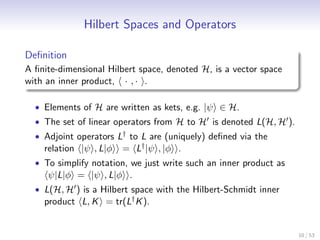
We use two metrics between quantum states:
Definition
The trace distance is defined as
1
∆(ρ, σ) := tr|ρ − σ| .
2
and the purified distance [TCR10] is defined as
P(ρ, σ) = 1 − F (ρ, σ).
√ √ 2
• The fidelity is F (ρ, σ) = tr| ρ σ| .
• Fuchs-van de Graaf Inequality [FvdG99]:
∆(ρ, σ) ≤ P(ρ, σ) ≤ 2∆(ρ, σ).
14 / 53

15. Completely Positive Maps
Definition
A completely positive map (CPM), E, is a linear map from L(HA )
to L(HB ) of the form
E :X → Lk XL† ,
k
k
where Lk are linear operators from HA to HB .
• CPMs map positive semi-definite operators onto positive
semi-definite operators.
• They are trace-preserving (TP) if tr(E(K )) = tr(K ) for all
K ∈ L(HA ).
• They are unital if E(1A ) = 1B .
• The adjoint map E † of E is defined through the relation
L, E(K ) = E † (L), K for all L ∈ L(H ), K ∈ L(H).
• The partial trace, trB , is the adjoint map to ρA → ρA ⊗ 1B .
15 / 53

16. Choi-Jamiolkowski Isomorphism
• The adjoint maps of trace-preserving maps are unital, and the
adjoint maps of unital maps are trace-preserving.
The Choi-Jamiolkowski isomorphism establishes a one-to-one
correspondence between CPMs from L(HA ) to L(HB ) and positive
semi-definite operators in L(HA ⊗ HB ).
E
cj : E → ωAB = EA →B |γAA γAA | , where |γAA = |ex ⊗ |ex
x
for some orthonormal basis {|ex }x of HA .
E
• Choi-Jamiolkowski states of TP CPMs satisfy trB ωAB = 1A .
• Choi-Jamiolkowski states of unital CPMs satisfy
E
trA ωAB = 1B .
16 / 53

17. Measurements
Definition
A positive operator-valued measure (POVM) on HA is a set {Mx }x
of operators Mx ≥ 0 such that x Mx = 1A .
• The associated measurement is the unital TP CPM
MX : ρAB → ρXB = |ex ex | ⊗ trA Mx ρAB Mx ,
x
where we omit 1B to shorten notation.
• The resulting state ρXB =
√ √ px |ex ex | ⊗ ρx is CQ with
x √ B √
px = tr Mx ρAB Mx and ρx = 1/px · Mx ρAB Mx .
B
• If all Mx satisfy (Mx )2 = Mx , the measurement is projective.
Moreover, if all Mx have rank 1, it is a rank-1 measurement.
17 / 53

18. The most important rule!
Lemma
For any CPM E, the following implication holds
A ≥ B =⇒ E(A) ≥ E(B).
Proof.
A ≥ B =⇒ A − B ≥ 0 =⇒ E(A − B) ≥ 0 =⇒ E(A) ≥ E(B).
• Example: A ≥ B =⇒ LAL† ≥ LBL† for any L.
18 / 53

19. Semi-Definite Programming
• We use the notation of Watrous [Wat08] and restrict to
positive operators.
Definition
A semi-definite program (SDP) is a triple {A, B, Ψ}, where A ≥ 0,
B ≥ 0 and Ψ a CPM. The following two optimization problems are
associated with the semi-definite program.
primal problem dual problem
minimize : A, X maximize : B, Y
subject to : Ψ(X ) ≥ B subject to : Ψ† (Y ) ≤ A
X ≥0 Y ≥0
• Under certain weak conditions, both optimizations evaluate to
the same value. (This is called strong duality.)
19 / 53

20. The Min-Entropy and Guessing
Now it gets more interesting.
20 / 53

21. Min-Entropy: Definition
Definition (Min-Entropy)
Let ρAB ∈ S(HAB ) be a quantum state. The min-entropy of A
conditioned on B of the state ρAB is
Hmin (A|B)ρ := sup λ ∈ R ∃σB ∈ S(HB ) : ρAB ≤ 2−λ 1A ⊗ σB .
• The supremum is bounded from above by log dim{HA }.
( ρAB ≤ 2−λ 1A ⊗ σB =⇒ 1 ≤ 2−λ dim{HA }. )
• Choosing σB = 1B / dim{HB }, we see that 2−λ = dim{HB } is
a lower bound.
• This implies − log dim{HB } ≤ Hmin (A|B)ρ ≤ log dim{HA }.
• The set is also closed, thus compact, and we can replace the
supremum by a maximum.
Question:
Nice, but how can I calculate this messy thing for a given state?
21 / 53

22. Min-Entropy: SDP I
Recall: Hmin (A|B)ρ = max λ ∈ R ∃σB ∈ S(HB ) : ρAB ≤ 2−λ 1A ⊗ σB
We can rewrite this as
2−Hmin (A|B)ρ = min µ ∈ R+ ∃σB ∈ S(HB ) : ρAB ≤ µ1A ⊗ σB .
Absorbing µ into σB , we can express 2−Hmin (A|B)ρ as the primal
problem of an SDP.
The primal problem for the min-entropy.
primal problem
minimize : 1B , σB
subject to : 1A ⊗ σB ≥ ρAB
σB ≥ 0
22 / 53

23. Min-Entropy: SDP II
Recall the primal problem for the min-entropy:
minimize : 1B , σ B
subject to : 1A ⊗ σB ≥ ρAB
σB ≥ 0
To find the dual program
• We introduce a dual variable XAB ≥ 0.
• We use Ψ : σB → 1A ⊗ σB . Then, Ψ† : XAB → trA (XAB ).
The SDP for the min-entropy.
primal problem dual problem
minimize : 1B , σB maximize : ρAB , XAB
subject to : 1A ⊗ σB ≥ ρAB subject to : XB ≤ 1B
σB ≥ 0 XAB ≥ 0
This SDP is strongly dual (without proof).
23 / 53

24. Min-Entropy: SDP III
Recall the SDP for the min-entropy:
minimize : 1B , σB maximize : ρAB , XAB
subject to : 1A ⊗ σB ≥ ρAB subject to : XB ≤ 1B
σB ≥ 0 XAB ≥ 0
• The dual optimal states will always satisfy XB = 1B .
• They correspond to Choi-Jamiolkowski states of unital CPMs
from A to B.
• Their adjoint maps are TP CPMs from B to A.
• We thus find the following expression for the min-entropy:
†
2−Hmin (A|B)ρ = max ρAB , EA →B (|γ γ|)
E†
= max γAA |EB→A (ρAB )|γAA ,
E
where we optimize over all TP CPMs EB→A from B to A ,
and fix |γAA = k |ek ⊗ |ek .
24 / 53

25. Guessing Probability
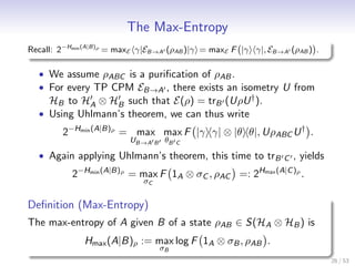
Recall: 2−Hmin (A|B)ρ = maxE γAA |EB→A (ρAB )|γAA .
• We consider a CQ state ρXB . Then, the expression simplifies
2−Hmin (X |B)ρ = max ey | ⊗ ey | px |ex ex | ⊗ E(ρx ) |ez ⊗ |ez
B
E
x,y ,z
= max px ex |E(ρx )|ex .
B
E
x
• The maximum is taken for maps of the form
E : ρB → x |ex ex | tr Mx ρB , where {Mx }x is a POVM.
Thus
2−Hmin (X |B)ρ = max px tr(Mx ρx )
B
{Mx }x
x
• This is the maximum probability of guessing X correctly for
an observer with access to the quantum system B [KRS09].
25 / 53

26. The Max-Entropy
Recall: 2−Hmin (A|B)ρ = maxE γ|EB→A (ρAB )|γ = maxE F |γ γ|, EB→A (ρAB ) .
• We assume ρABC is a purification of ρAB .
• For every TP CPM EB→A , there exists an isometry U from
HB to HA ⊗ HB such that E(ρ) = trB (UρU † ).
• Using Uhlmann’s theorem, we can thus write
2−Hmin (A|B)ρ = max max F |γ γ| ⊗ |θ θ|, UρABC U † .
UB→A B θB C
• Again applying Uhlmann’s theorem, this time to trB C , yields
2−Hmin (A|B)ρ = max F 1A ⊗ σC , ρAC =: 2Hmax (A|C )ρ .
σC
Definition (Max-Entropy)
The max-entropy of A given B of a state ρAB ∈ S(HA ⊗ HB ) is
Hmax (A|B)ρ := max log F 1A ⊗ σB , ρAB .
σB
26 / 53

27. Examples I
• For a pure state ρAB = |ψ ψ| in Schmidt decomposition
√
|ψAB = i µi |ei ⊗ |ei , we get ρA = i µi |ei ei | and
Hmin (A|B)ρ = −Hmax (A)ψ = − log F (1A , ρA )
√ 2
= − log µi .
i
1
• For a maximally entangled state, µi = d , and
Hmin (A|B)ρ = − log d .
• This is also evident from the expression
Hmin (A|B)ρ = − log max F |γ γ|, EB→A (ρAB )
E
1
as |ψ = √ |γ
d
is already of the required form.
27 / 53

28. Examples II
Recall the SDP for the min-entropy:
minimize : 1B , σB maximize : ρAB , XAB
subject to : 1A ⊗ σB ≥ ρAB subject to : XB ≤ 1B
σB ≥ 0 XAB ≥ 0
• Take product states ρAB = ρA ⊗ ρB with ρA = x µx |ex ex |,
and µ1 ≥ µ2 ≥ . . . ≥ µk .
• We choose σB = µ1 ρB and XAB = |e1 e1 | ⊗ 1B .
• Clearly, 1A ⊗ σB ≥ ρA ⊗ ρB since µ1 1A ≥ ρA . Hence, σB and
XAB are feasible.
• This gives us lower and upper bounds on the min-entropy
µ1 = ρAB , XAB ≤ 2−Hmin (A|B)ρ ≤ 1B , σB = µ1 .
• Finally, note that Hmin (A|B)ρ = − log µ1 = Hmin (A)ρ .
28 / 53

29. Is the Min-Entropy a R´nyi-Entropy?
e
• Yes (ongoing work with Oleg Szehr and Fr´d´ric Dupuis), the
e e
R´nyi-Entropies
e
α
Hα (A)ρ := log ρA α
1−α
can be generalized to
α ρAB
Hα (A|B)ρ,σ := log ,
1−α σB α,1A ⊗σB
1 1
where ρAB = (1A ⊗ σB )− 2 ρAB (1A ⊗ σB )− 2 and we use the
σB
weighted norms
1
1 1 α α
ρ α,τ := tr τ 2α ρ τ 2α .
• Now, Hmin (A|B)ρ = maxσB limn→∞ Hα (A|B)ρ,σ
• And Hmax (A|B)ρ = maxσB H 1 (A|B)ρ,σ .
2
29 / 53

30. Smooth Min- and Max-Entropies
And their operational interpretation.
30 / 53

31. Why Smoothing?
1. Most properties of the min- and max-entropy generalize to
smooth entropies.
2. On top of that, the smooth entropies have additional
properties. Most prominently, they satisfy an entropic
equipartition law which relates them to the conditional von
Neumann entropy.
3. The smoothing parameter has operational meaning in some
applications, for example, the ε-smooth min-entropy
characterizes how much ε-close to uniform randomness can be
extracted from a random variable.
4. The smooth entropies allow us to exclude improbable events.
A statistical analysis performed on a random sample of states
may thus allow us to bound a smooth entropy, but not
(directly) the actual min- or max-entropy.
31 / 53

32. A Ball of ε-Close States
Recall: P(ρ, τ ) := 1 − F (ρ, τ ), where F is the fidelity.
• We write ρ ≈ε τ if P(ρ, τ ) ≤ ε.
• The purified distance has a triangle inequality
P(ρ, σ) ≤ P(ρ, τ ) + P(τ, σ).
• The purified distance is contractive under TP CPMs E and
projections Π, Π2 = Π:
ρ ≈ε τ =⇒ E(ρ) ≈ε E(τ ) ∧ ΠρΠ ≈ε Πτ Π .
• For two states ρA ≈ε τA a state ρAB with trB (ρAB ) = ρA ,
there exists a state τAB with trB (τAB ) = τA and τAB ≈ε ρAB .
• We define a ball of ε-close states around ρ as
B ε (ρ) := ρ ≥ 0 ρ ≈ε ρ ∧ tr(˜) ≤ 1 .
˜ ˜ ρ
32 / 53

33. Smooth Entropies
Definition (Smooth Entropies [TCR10])
Let 0 ≤ ε < 1 and ρAB ∈ S(HA ⊗ HB ). The ε-smooth
min-entropy of A given B is defined as
ε
Hmin (A|B)ρ := max Hmin (A|B)ρ .
˜
ρAB ∈B ε (ρAB )
˜
The ε-smooth max-entropy of A given B is defined as
ε
Hmax (A|B)ρ := min Hmax (A|B)ρ .
˜
ρAB ∈B ε (ρAB )
˜
ε ε
• They satisfy a duality relation: Hmax (A|B)ρ = −Hmin (A|C )ρ
for any pure state ρABC .
33 / 53

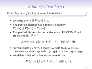
34. Operational Interpretation: Smooth Min-Entropy I
• Investigate the maximum number of random and independent
bits that can be extracted from a CQ random source ρXE .
• A protocol P extracts a random number Z from X .
ε
(X |E )ρ :=
max ∈ N ∃ P, σE : |Z | = 2 ∧ ρZE ≈ε 2− 1Z ⊗ σE .
ε
• Renner [Ren05] showed that Hmin (A|B) can be extracted, up
to terms logarithmic in ε, and a converse was shown for ε = 0.
• We recently showed a stronger result [TH12]
ε ε ε−η 1
Hmin (X |E )ρ ≥ (X |E )ρ ≥ Hmin (X |E )ρ − 4 log − 3.
η
• The smoothing parameter, ε, thus has operational meaning as
the allowed distance from perfectly secret randomness.
34 / 53

35. Operational Interpretation: Smooth Min-Entropy II
Recall: 0
(X |E )ρ = max ∈ N ∃ P, σE : |Z | = 2 ∧ ρZE = 2− 1Z ⊗ σE .
• To get some intuition, we can consider the case ε = 0.
• We now show that Hmin (X |E )ρ ≥ 0 (X |E )ρ , i.e. that the
number of perfectly secret bits that can be extracted from X
is bounded by the conditional min-entropy of X given E .
Proof.
• By definition, the protocol must output a state of the form
0 (X |E )
ρZE = 2− 1Z ⊗ σE . Hence, pguess (Z |E )ρ = 2− ≤ 2− ρ .
• Since Z = f (X ) is the output of a function, and since it is
harder to guess the input of a function than its output, we get
pguess (Z |E )ρ ≥ pguess (X |E )ρ .
• Thus,
Hmin (X |E )ρ = − log pguess (X |E )ρ
0
≥ − log pguess (Z |E )ρ ≥ (X |E )ρ .
35 / 53

36. Operational Interpretation: Smooth Max-Entropy
• Find the minimum encoding length for data reconciliation of
X if quantum side information B is available.
• A protocol P encodes X into M and then produces an
estimate X of X from B and M.
mε (X |E )ρ := min m ∈ N ∃P : |M| = 2m ∧ P[X = X ] ≤ ε .
• Renes and Renner [RR12] showed that
√ 1
Hmax (X |B)ρ ≤ mε (X |B)ρ ≤ Hmax (X |B)ρ + 2 log
2ε ε−η
+ 4.
η
• The smoothing parameter, ε, is related to the allowed
decoding error probability.
36 / 53

37. Basic Properties of Smooth Entropies
37 / 53

38. Asymptotic Equipartition
• Classically, for n independent and identical (i.i.d.) repetitions
of a task, we consider a random variable X n = (X1 , . . . , Xn )
and a probability distribution P[X n = x n ] = i P[Xi = xi ].
• Then, − log P(x n ) → H(X ) in probability for n → ∞.
• This means that the distribution is essentially flat, and since
smoothing removes “untypical” events, all entropies converge
to the Shannon entropy.
Theorem (Entropic Asymptotic Equipartition [TCR09])
Let 0 < ε < 1 and ρAB ∈ S(HA ⊗ HB ). Then, the sequence of
states {ρn }n , with ρn = ρ⊗n , satisfies
AB AB AB
1 ε 1 ε
lim H (A|B)ρn = lim Hmax (A|B)ρn = H(A|B)ρ .
n→∞ n min n→∞ n
38 / 53

39. Data-Processing Inequalities
• Operations on the observers (quantum) memory cannot
decrease the uncertainty about the system.
• We consider a TP CPM E from B to B . This maps the state
ρAB to τAB = E(ρAB ) and
ε ε ε ε
Hmin (A|B )τ ≥ Hmin (A|B)ρ , Hmax (A|B )τ ≥ Hmax (A|B)ρ .
• An additional register K with k bits of classical information
cannot decrease the uncertainty by more than k. Thus,
ε ε
Hmin (A|BK ) ≥ Hmin (A|B) − k ,
ε ε
Hmax (A|BK ) ≥ Hmax (A|B) − k .
39 / 53

40. Data-Processing Inequalities II
Theorem (Data-Processing for Min-Entropy)
Let 0 ≤ ε < 1, ρAB ∈ S(HA ⊗ HB ), and E a TP CPM from B to
B with τAB = E(ρAB ). Then,
ε ε
Hmin (A|B )τ ≥ Hmin (A|B)ρ .
Recall: Hmin (A|B)ρ = max λ ∃σB , ρAB : ρAB ≈ε ρAB ∧ ρAB ≤ 2−λ 1A ⊗ σB .
ε
˜ ˜ ˜
ε
• Set λ = Hmin (A|B)ρ . Then, by definition there exists a state
ρAB ≈ε ρAB and a state σB ∈ S(HB ) such that
˜
ρAB ≤ 2−λ 1A ⊗ σB =⇒ E(˜AB ) ≤ 2−λ 1A ⊗ E(σB ) .
˜ ρ
• Contractivity: E(˜AB ) ≈ε τAB . Also, E(σB ) ∈ S(HB ).
ρ
ε (A|B ) ≥ λ.
• Thus, Hmin τ
40 / 53

41. Entropic Uncertainty I
Given Θ, what is X?
O1
Θ ∈ {+, ×}
uniform
ρ O2
X
• The observers, Bob (O1 ) and Charlie (O2 ), prepare a tripartite
quantum state, shared with Alice. (This can be an arbitrary
state ρABC .)
• Alice measures her system in a basis determined by Θ.
• What is the entropy the observers have about the outcome X ,
after they are given Θ?
41 / 53

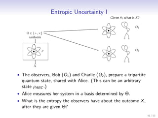
42. Entropic Uncertainty II
Apply measurement in a basis determined by a uniform θ ∈ {0, 1}.
Theorem (Entropic Uncertainty Relation [TR11, Tom12])
θ
For any state ρABC , ε ≥ 0 and POVMs {Mx } on A, Θ uniform:
ε ε 1
Hmin (X |BΘ) + Hmax (X |C Θ) ≥ log ,
c
2
c = max 0
Mx 1
Mx ,
x,y ∞
θ
ρXBC Θ = |ex ex | ⊗ |eθ eθ | ⊗ trA (Mx ⊗ 1BC )ρABC .
x,θ
2
• Overlap is c = maxx,y x 0 |y 1 for projective measurements,
where |x 0 is an eigenvector of Mx and |y 1 is an eigenvector
0
1
of Mx .
• For example, for qubit measurements in the computational
1
and Hadamard basis: c = 2 .
42 / 53

43. Entropic Uncertainty III
• This can be lifted to n independent measurements, each
chosen at random.
1
Hmin (X n |BΘn ) + Hmax (X n |C Θn ) ≥ n log .
ε ε
c
• This implies previous uncertainty relations for the von
Neumann entropy [BCC+ 10] via asymptotic equipartition.
• For this, we apply the above relation to product states
ρn = ρ⊗n .
ABC ABC
• Then, we divide by n and use
1 ε n→∞
H (X n |B n Θn ) − − → H(X |BΘ) .
−−
n min/max
1
This yields H(X |BΘ) + H(X |C Θ) ≥ log c in the limit.
43 / 53

44. Quantum Key Distribution
An attempt to prove security on 4 slides.
(Asymptotically, and trusting our devices to some degree...)
44 / 53

45. Protocol
• We consider the entanglement-based Bennett-Brassard 1984
protocol [BBM92].
• We only do an asymptotic analysis here, a finite-key analysis
based on this method can be found in [TLGR12].
• Alice produces n pairs of entangled qubits, and sends one
qubit of each pair to Bob. This results in a state ρAn B n E .
• Then, Alice randomly chooses a measurement basis for each
qubit, either + or ×, and records her measurement outcomes
in X n . She sends the string of choices, Θn , to Bob.
• ˆ
Bob, after learning Θn , produces an estimate X n of X n by
measuring the n systems he received.
• Alice and Bob calculate the error rate δ on a random sample.
• Then, classical information reconciliation and privacy
amplification protocols are employed to extract a shared secret
ˆ
key Z from the raw keys, X n and X n .
• We are interested in the secret key rate.
45 / 53

46. Security Analysis I
• Consider the situation before Bob measures
ρX n B n E = |x n x n | ⊗ trAn θ
Pxii ⊗ 1B n E ρAn B n E ,
xn
where Px = H θ |ex ex |H θ and H the Hadamard matrix.
θ
• The uncertainty relation applies here,
1
Hmin (X n |E Θn ) + Hmax (X n |B n Θn ) ≥ n log
ε ε
= n.
c
• Data-Processing of the smooth max-entropy then implies
ε ε ˆ
Hmin (X n |E Θn ) ≥ n − Hmax (X n |X n ),
ˆ
since X n is the result of a TP CPM applied to B n and Θn .
46 / 53

47. Security Analysis II
ε ε ˆ
Recall: Hmin (X n |E Θn ) ≥ n − Hmax (X n |X n ).
• Let ε be a small constant.
• The extractable ε-secure key length is give by ε (X n |E ΘSP),
where S is the syndrom Alice sends to Bob for error correction
and P is the information leaked due to parameter estimation.
• We ignore P for this analysis, and just note that
log |P| = o(n).
• If we want information reconciliation up to probability ε, we
ˆ
can bound log |S| ≤ Hmax (X n |X n ) + O(1) using the
ε
operational interpretation of the smooth max-entropy.
• This ensures that
ε
(X n |E ΘSP) ≥ Hmin (X n |E ΘSP) + O(1)
ε
ε ε ˆ
≥ Hmin (X n |E Θ) − Hmax (X n |X n ) + o(n)
ˆ
≥ n − 2Hmax (X n |X n ) + o(n).
ε
47 / 53

48. Security Analysis III
Recall: ε ˆ
(X n |E ΘSP) ≥ n − 2Hmax (X n |X n ) + o(n) .
ε
• We have now reduced the problem of bounding Eve’s
information about the key to bounding the correlations
between Alice and Bob.
• From the observed error rate δ, we can estimate the smooth
ˆ
max-entropy: Hmax (X n |X n ) ≤ nh(δ), where h is the binary
ε
entropy. (This one you just have to believe me.)
• The secret key rate thus asymptotically approaches
1 ε n
r = lim (X |E ΘSP) ≥ n 1 − 2h(δ) .
n→∞ n
• This recovers the results due to Mayers [May96, May02], and
Shor and Preskill [SP00].
48 / 53

49. Conclusion
• The entropic approach to quantum information is very
powerful, especially in cryptography.
• The smooth entropies are universal, they have many useful
properties (I discussed only a small fraction of them here) and
clear operational meaning.
• The smooth entropy formalism leads to an intuitive security
proof for QKD, which also naturally yields finite key bounds.
49 / 53

50. Thank you for your attention.
50 / 53

51. Bibliography I
[BBM92] Charles H. Bennett, Gilles Brassard, and N. D. Mermin, Quantum cryptography without Bells
theorem, Phys. Rev. Lett. 68 (1992), no. 5, 557–559.
[BCC+ 10] Mario Berta, Matthias Christandl, Roger Colbeck, Joseph M. Renes, and Renato Renner, The
Uncertainty Principle in the Presence of Quantum Memory, Nat. Phys. 6 (2010), no. 9, 659–662.
[BD10] Francesco Buscemi and Nilanjana Datta, The Quantum Capacity of Channels With Arbitrarily
Correlated Noise, IEEE Trans. on Inf. Theory 56 (2010), no. 3, 1447–1460.
[Ber08] Mario Berta, Single-Shot Quantum State Merging, Master’s thesis, ETH Zurich, 2008.
[Col12] Patrick J. Coles, Collapse of the quantum correlation hierarchy links entropic uncertainty to
entanglement creation.
[Dat09] Nilanjana Datta, Min- and Max- Relative Entropies and a New Entanglement Monotone, IEEE Trans.
on Inf. Theory 55 (2009), no. 6, 2816–2826.
[DBWR10] Fr´d´ric Dupuis, Mario Berta, J¨rg Wullschleger, and Renato Renner, The Decoupling Theorem.
e e u
[dRAR+ 11] L´
ıdia del Rio, Johan Aberg, Renato Renner, Oscar Dahlsten, and Vlatko Vedral, The Thermodynamic
Meaning of Negative Entropy., Nature 474 (2011), no. 7349, 61–3.
[DrFSS08] Ivan B. Damg˚ rd, Serge Fehr, Louis Salvail, and Christian Schaffner, Cryptography in the
a
Bounded-Quantum-Storage Model, SIAM J. Comput. 37 (2008), no. 6, 1865.
[DRRV11] Oscar C O Dahlsten, Renato Renner, Elisabeth Rieper, and Vlatko Vedral, Inadequacy of von
Neumann Entropy for Characterizing Extractable Work, New J. Phys. 13 (2011), no. 5, 053015.
[Dup09] Fr´d´ric Dupuis, The Decoupling Approach to Quantum Information Theory, Ph.D. thesis, Universit´
e e e
de Montr´al, April 2009.
e
[FvdG99] C.A. Fuchs and J. van de Graaf, Cryptographic distinguishability measures for quantum-mechanical
states, IEEE Trans. on Inf. Theory 45 (1999), no. 4, 1216–1227.
51 / 53

52. Bibliography II
[KRS09] Robert K¨nig, Renato Renner, and Christian Schaffner, The Operational Meaning of Min- and
o
Max-Entropy, IEEE Trans. on Inf. Theory 55 (2009), no. 9, 4337–4347.
[KWW12] Robert Konig, Stephanie Wehner, and J¨rg Wullschleger, Unconditional Security From Noisy
u
Quantum Storage, IEEE Trans. on Inf. Theory 58 (2012), no. 3, 1962–1984.
[May96] Dominic Mayers, Quantum Key Distribution and String Oblivious Transfer in Noisy Channels, Proc.
CRYPTO, LNCS, vol. 1109, Springer, 1996, pp. 343–357.
[May02] , Shor and Preskill’s and Mayers’s security proof for the BB84 quantum key distribution
protocol, Eur. Phys. J. D 18 (2002), no. 2, 161–170.
[R´n61]
e A. R´nyi, On Measures of Information and Entropy, Proc. Symp. on Math., Stat. and Probability
e
(Berkeley), University of California Press, 1961, pp. 547–561.
[Ren05] Renato Renner, Security of Quantum Key Distribution, Ph.D. thesis, ETH Zurich, December 2005.
[RK05] Renato Renner and Robert K¨nig, Universally Composable Privacy Amplification Against Quantum
o
Adversaries, Proc. TCC (Cambridge, USA), LNCS, vol. 3378, 2005, pp. 407–425.
[RR12] Joseph M. Renes and Renato Renner, One-Shot Classical Data Compression With Quantum Side
Information and the Distillation of Common Randomness or Secret Keys, IEEE Trans. on Inf. Theory
58 (2012), no. 3, 1985–1991.
[Sha48] C. Shannon, A Mathematical Theory of Communication, Bell Syst. Tech. J. 27 (1948), 379–423.
[SP00] Peter Shor and John Preskill, Simple Proof of Security of the BB84 Quantum Key Distribution
Protocol, Phys. Rev. Lett. 85 (2000), no. 2, 441–444.
[TCR09] Marco Tomamichel, Roger Colbeck, and Renato Renner, A Fully Quantum Asymptotic Equipartition
Property, IEEE Trans. on Inf. Theory 55 (2009), no. 12, 5840–5847.
52 / 53

53. Bibliography III
[TCR10] , Duality Between Smooth Min- and Max-Entropies, IEEE Trans. on Inf. Theory 56 (2010),
no. 9, 4674–4681.
[TH12] Marco Tomamichel and Masahito Hayashi, A Hierarchy of Information Quantities for Finite Block
Length Analysis of Quantum Tasks.
[TLGR12] Marco Tomamichel, Charles Ci Wen Lim, Nicolas Gisin, and Renato Renner, Tight Finite-Key
Analysis for Quantum Cryptography, Nat. Commun. 3 (2012), 634.
[Tom12] Marco Tomamichel, A Framework for Non-Asymptotic Quantum Information Theory, Ph.D. thesis,
ETH Zurich, March 2012.
[TR11] Marco Tomamichel and Renato Renner, Uncertainty Relation for Smooth Entropies, Phys. Rev. Lett.
106 (2011), no. 11.
[Wat08] John Watrous, Theory of Quantum Information, Lecture Notes, 2008.
[WTHR11] Severin Winkler, Marco Tomamichel, Stefan Hengl, and Renato Renner, Impossibility of Growing
Quantum Bit Commitments, Phys. Rev. Lett. 107 (2011), no. 9.
[WW08] Stephanie Wehner and J¨rg Wullschleger, Composable Security in the Bounded-Quantum-Storage
u
Model, Proc. ICALP, LNCS, vol. 5126, Springer, July 2008, pp. 604–615.
[WW12] Severin Winkler and J¨rg Wullschleger, On the Efficiency of Classical and Quantum Secure Function
u
Evaluation.
53 / 53