Download as PDF, PPTX


![Having Latent Variables Log-Liklihood of MRF
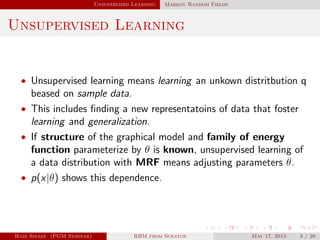
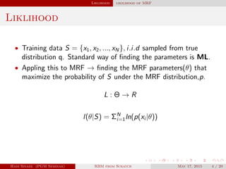
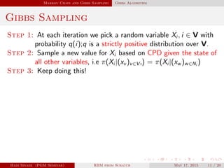
• Log-Liklihood for one sample:
l(θ|v) = ln[Σhe−E(v,h)
] − ln[
Z
Σv,he−E(v,h)
]
Hadi Sinaee (PGM Seminar) RBM from Scratch May 17, 2015 8 / 20](https://image.slidesharecdn.com/rbm-150703072830-lva1-app6892/85/RBM-from-Scratch-23-320.jpg)
![Having Latent Variables Log-Liklihood of MRF
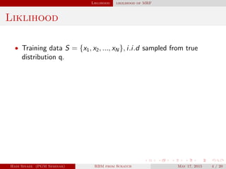
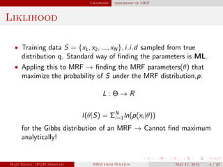
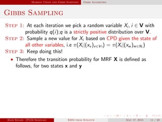
• Log-Liklihood for one sample:
l(θ|v) = ln[Σhe−E(v,h)
] − ln[
Z
Σv,he−E(v,h)
]
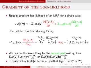
• Then its gradient is:
θl = −Σhp(h|v)
∂E(v, h)
∂θ
+ Σv,hp(v, h)
∂E(v, h)
∂θ
Hadi Sinaee (PGM Seminar) RBM from Scratch May 17, 2015 8 / 20](https://image.slidesharecdn.com/rbm-150703072830-lva1-app6892/85/RBM-from-Scratch-24-320.jpg)
![Having Latent Variables Log-Liklihood of MRF
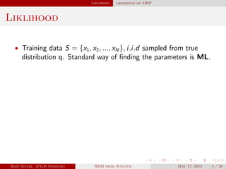
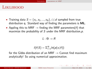
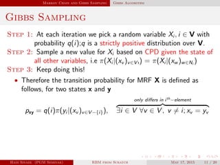
• Log-Liklihood for one sample:
l(θ|v) = ln[Σhe−E(v,h)
] − ln[
Z
Σv,he−E(v,h)
]
• Then its gradient is:
θl = −Σhp(h|v)
∂E(v, h)
∂θ
+ Σv,hp(v, h)
∂E(v, h)
∂θ
• It is difference of two expectations:
Hadi Sinaee (PGM Seminar) RBM from Scratch May 17, 2015 8 / 20](https://image.slidesharecdn.com/rbm-150703072830-lva1-app6892/85/RBM-from-Scratch-25-320.jpg)
![Having Latent Variables Log-Liklihood of MRF
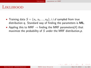
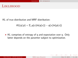
• Log-Liklihood for one sample:
l(θ|v) = ln[Σhe−E(v,h)
] − ln[
Z
Σv,he−E(v,h)
]
• Then its gradient is:
θl = −Σhp(h|v)
∂E(v, h)
∂θ
+ Σv,hp(v, h)
∂E(v, h)
∂θ
• It is difference of two expectations:
→One over conditional dist. of hidden units
Hadi Sinaee (PGM Seminar) RBM from Scratch May 17, 2015 8 / 20](https://image.slidesharecdn.com/rbm-150703072830-lva1-app6892/85/RBM-from-Scratch-26-320.jpg)
![Having Latent Variables Log-Liklihood of MRF
• Log-Liklihood for one sample:
l(θ|v) = ln[Σhe−E(v,h)
] − ln[
Z
Σv,he−E(v,h)
]
• Then its gradient is:
θl = −Σhp(h|v)
∂E(v, h)
∂θ
+ Σv,hp(v, h)
∂E(v, h)
∂θ
• It is difference of two expectations:
→One over conditional dist. of hidden units
→One over model dist.
• We have to sum over all possible values of (v,h) for this
computation!!
Hadi Sinaee (PGM Seminar) RBM from Scratch May 17, 2015 8 / 20](https://image.slidesharecdn.com/rbm-150703072830-lva1-app6892/85/RBM-from-Scratch-27-320.jpg)
![Having Latent Variables Log-Liklihood of MRF
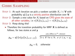
• Log-Liklihood for one sample:
l(θ|v) = ln[Σhe−E(v,h)
] − ln[
Z
Σv,he−E(v,h)
]
• Then its gradient is:
θl = −Σhp(h|v)
∂E(v, h)
∂θ
+ Σv,hp(v, h)
∂E(v, h)
∂θ
• It is difference of two expectations:
→One over conditional dist. of hidden units
→One over model dist.
• We have to sum over all possible values of (v,h) for this
computation!! Instead approximating this expectation.
Hadi Sinaee (PGM Seminar) RBM from Scratch May 17, 2015 8 / 20](https://image.slidesharecdn.com/rbm-150703072830-lva1-app6892/85/RBM-from-Scratch-28-320.jpg)
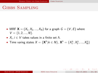
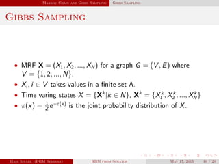
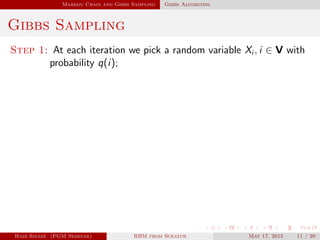
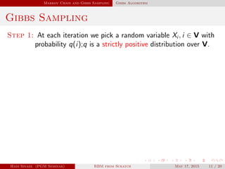
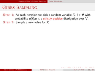
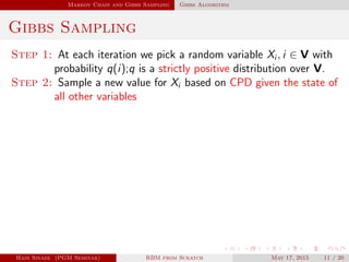
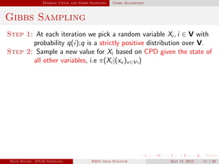
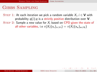
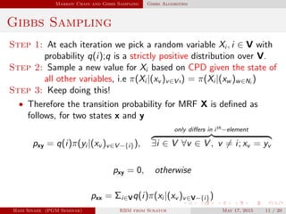


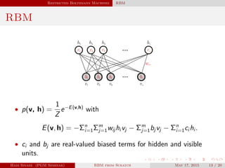
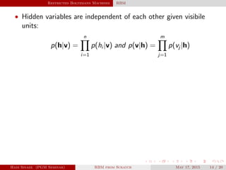
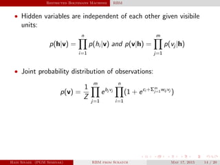
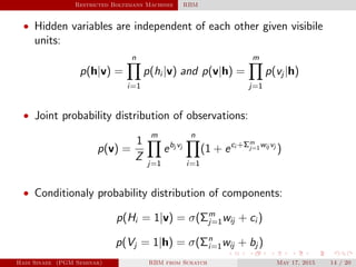
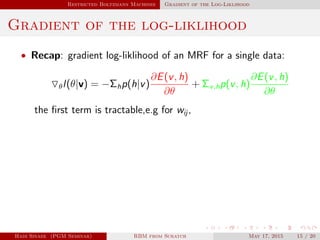
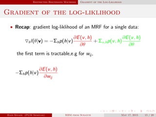
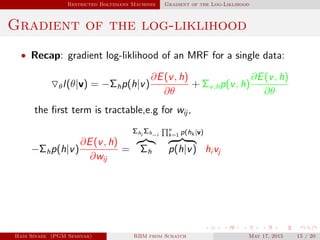
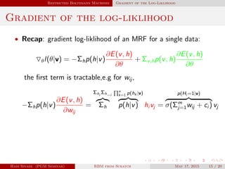
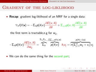
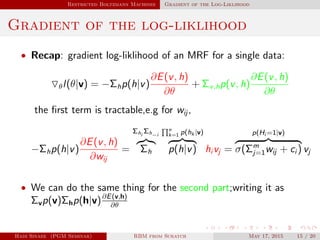
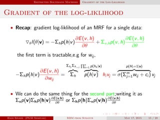
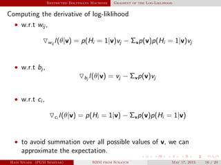
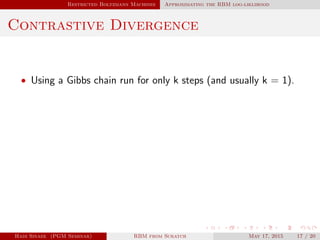
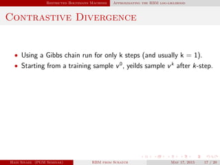
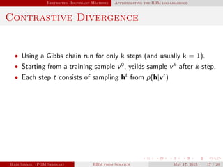
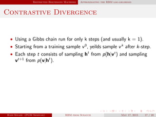
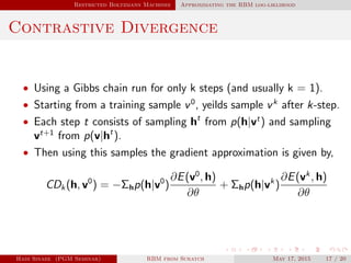
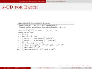
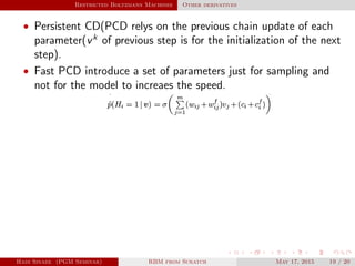
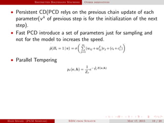
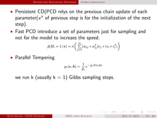
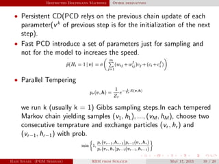

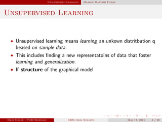
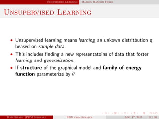
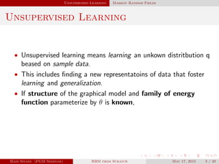
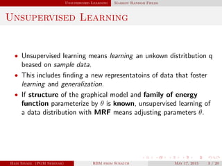
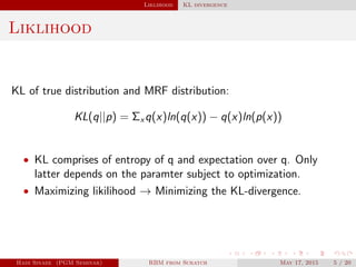
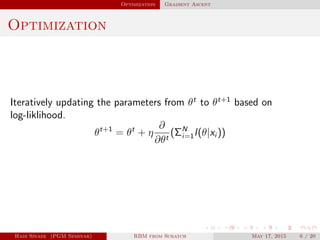
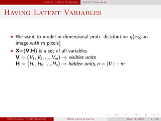
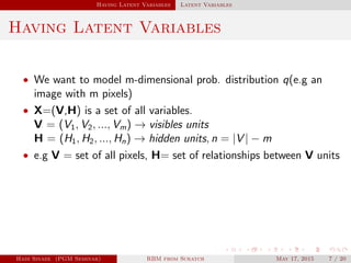
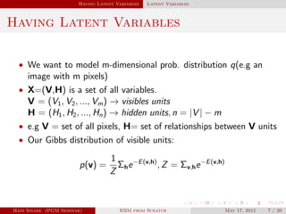
This document outlines Hadi Sinaee's seminar on Restricted Boltzmann Machines (RBMs) from scratch. The seminar covers: 1. Unsupervised learning and using Markov Random Fields (MRFs) to learn unknown data distributions. 2. Maximum likelihood estimation cannot be done analytically for MRFs, so numerical approximation is required. 3. Introducing latent variables in the form of hidden units allows modeling high-dimensional distributions like images. 4. Computing the log-likelihood gradient involves taking expectations that require summing over all possible latent variable assignments, so approximation is needed.