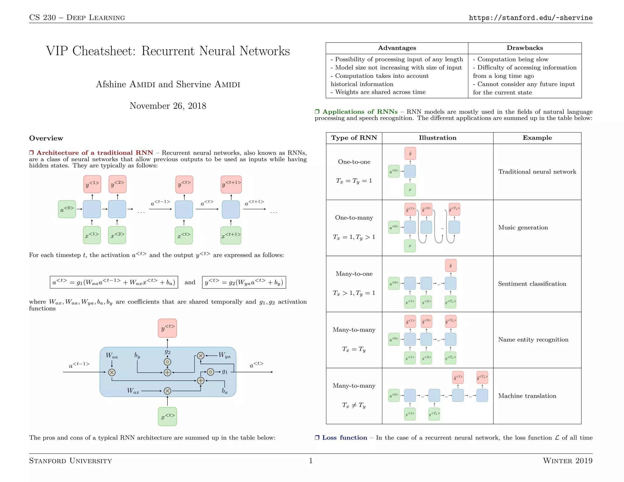
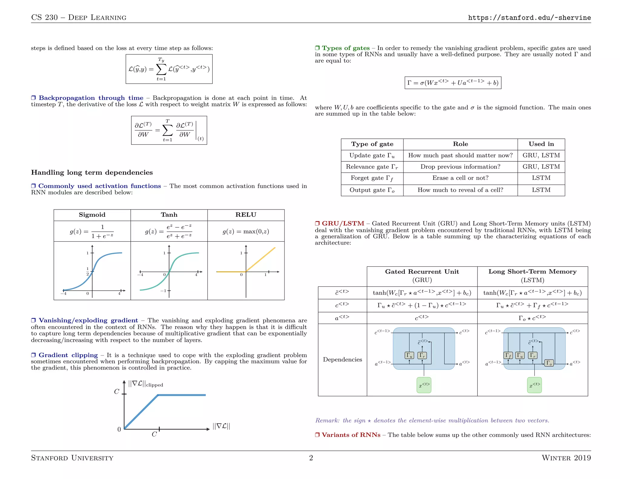
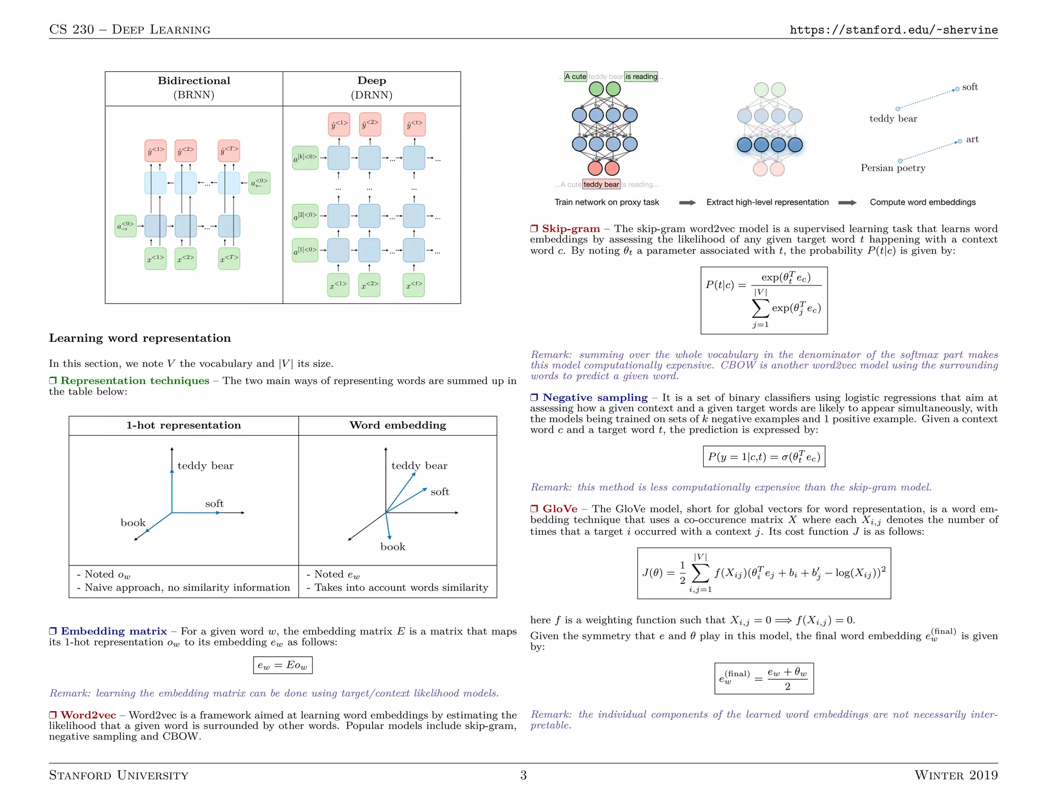
1. Recurrent neural networks (RNNs) allow information to persist from previous time steps through hidden states and can process input sequences of variable lengths. Common RNN architectures include LSTMs and GRUs which address the vanishing gradient problem of traditional RNNs. 2. RNNs are commonly used for natural language processing tasks like machine translation, sentiment classification, and named entity recognition. They learn distributed word representations through techniques like word2vec, GloVe, and negative sampling. 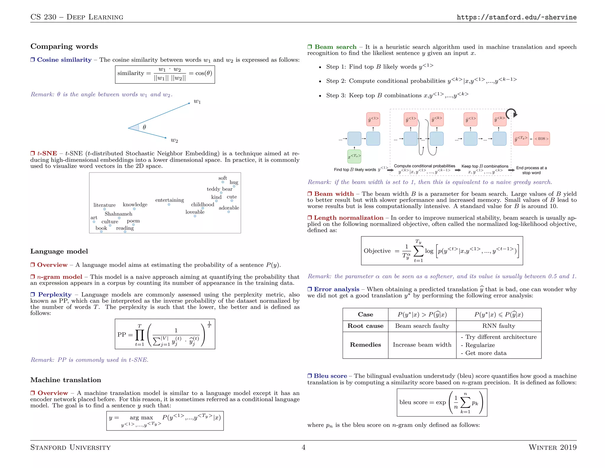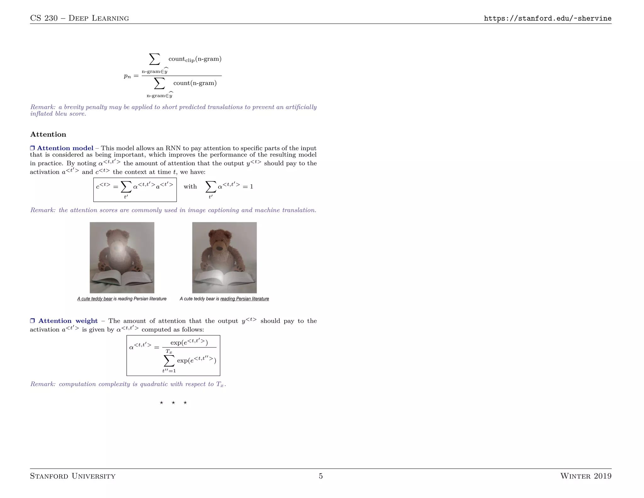3. Machine translation models use an encoder-decoder architecture with an RNN encoder and decoder. Beam search is commonly used to find high-probability translation sequences. Performance is evaluated using metrics like BLEU score.

1. CS 230 – Deep Learning https://stanford.edu/~shervine
VIP Cheatsheet: Recurrent Neural Networks
Afshine Amidi and Shervine Amidi
November 26, 2018
Overview
r Architecture of a traditional RNN – Recurrent neural networks, also known as RNNs,
are a class of neural networks that allow previous outputs to be used as inputs while having
hidden states. They are typically as follows:
For each timestep t, the activation a<t> and the output y<t> are expressed as follows:
a<t>
= g1(Waaa<t−1>
+ Waxx<t>
+ ba) and y<t>
= g2(Wyaa<t>
+ by)
where Wax, Waa, Wya, ba, by are coefficients that are shared temporally and g1, g2 activation
functions
The pros and cons of a typical RNN architecture are summed up in the table below:
Advantages Drawbacks
- Possibility of processing input of any length
- Model size not increasing with size of input
- Computation takes into account
historical information
- Weights are shared across time
- Computation being slow
- Difficulty of accessing information
from a long time ago
- Cannot consider any future input
for the current state
r Applications of RNNs – RNN models are mostly used in the fields of natural language
processing and speech recognition. The different applications are summed up in the table below:
Type of RNN Illustration Example
One-to-one
Tx = Ty = 1
Traditional neural network
One-to-many
Tx = 1, Ty > 1
Music generation
Many-to-one
Tx > 1, Ty = 1
Sentiment classification
Many-to-many
Tx = Ty
Name entity recognition
Many-to-many
Tx 6= Ty
Machine translation
r Loss function – In the case of a recurrent neural network, the loss function L of all time
Stanford University 1 Winter 2019

2. CS 230 – Deep Learning https://stanford.edu/~shervine
steps is defined based on the loss at every time step as follows:
L(b
y,y) =
Ty
X
t=1
L(b
y<t>
,y<t>
)
r Backpropagation through time – Backpropagation is done at each point in time. At
timestep T, the derivative of the loss L with respect to weight matrix W is expressed as follows:
∂L(T )
∂W
=
T
X
t=1
∂L(T )
∂W

6. (t)
Handling long term dependencies
r Commonly used activation functions – The most common activation functions used in
RNN modules are described below:
Sigmoid Tanh RELU
g(z) =
1
1 + e−z
g(z) =
ez − e−z
ez + e−z
g(z) = max(0,z)
r Vanishing/exploding gradient – The vanishing and exploding gradient phenomena are
often encountered in the context of RNNs. The reason why they happen is that it is difficult
to capture long term dependencies because of multiplicative gradient that can be exponentially
decreasing/increasing with respect to the number of layers.
r Gradient clipping – It is a technique used to cope with the exploding gradient problem
sometimes encountered when performing backpropagation. By capping the maximum value for
the gradient, this phenomenon is controlled in practice.
r Types of gates – In order to remedy the vanishing gradient problem, specific gates are used
in some types of RNNs and usually have a well-defined purpose. They are usually noted Γ and
are equal to:
Γ = σ(Wx<t>
+ Ua<t−1>
+ b)
where W, U, b are coefficients specific to the gate and σ is the sigmoid function. The main ones
are summed up in the table below:
Type of gate Role Used in
Update gate Γu How much past should matter now? GRU, LSTM
Relevance gate Γr Drop previous information? GRU, LSTM
Forget gate Γf Erase a cell or not? LSTM
Output gate Γo How much to reveal of a cell? LSTM
r GRU/LSTM – Gated Recurrent Unit (GRU) and Long Short-Term Memory units (LSTM)
deal with the vanishing gradient problem encountered by traditional RNNs, with LSTM being
a generalization of GRU. Below is a table summing up the characterizing equations of each
architecture:
Gated Recurrent Unit
(GRU)
Long Short-Term Memory
(LSTM)
c̃<t> tanh(Wc[Γr ? a<t−1>,x<t>] + bc) tanh(Wc[Γr ? a<t−1>,x<t>] + bc)
c<t> Γu ? c̃<t> + (1 − Γu) ? c<t−1> Γu ? c̃<t> + Γf ? c<t−1>
a<t> c<t> Γo ? c<t>
Dependencies
Remark: the sign ? denotes the element-wise multiplication between two vectors.
r Variants of RNNs – The table below sums up the other commonly used RNN architectures:
Stanford University 2 Winter 2019

7. CS 230 – Deep Learning https://stanford.edu/~shervine
Bidirectional
(BRNN)
Deep
(DRNN)
Learning word representation
In this section, we note V the vocabulary and |V | its size.
r Representation techniques – The two main ways of representing words are summed up in
the table below:
1-hot representation Word embedding
- Noted ow
- Naive approach, no similarity information
- Noted ew
- Takes into account words similarity
r Embedding matrix – For a given word w, the embedding matrix E is a matrix that maps
its 1-hot representation ow to its embedding ew as follows:
ew = Eow
Remark: learning the embedding matrix can be done using target/context likelihood models.
r Word2vec – Word2vec is a framework aimed at learning word embeddings by estimating the
likelihood that a given word is surrounded by other words. Popular models include skip-gram,
negative sampling and CBOW.
r Skip-gram – The skip-gram word2vec model is a supervised learning task that learns word
embeddings by assessing the likelihood of any given target word t happening with a context
word c. By noting θt a parameter associated with t, the probability P(t|c) is given by:
P(t|c) =
exp(θT
t ec)
|V |
X
j=1
exp(θT
j ec)
Remark: summing over the whole vocabulary in the denominator of the softmax part makes
this model computationally expensive. CBOW is another word2vec model using the surrounding
words to predict a given word.
r Negative sampling – It is a set of binary classifiers using logistic regressions that aim at
assessing how a given context and a given target words are likely to appear simultaneously, with
the models being trained on sets of k negative examples and 1 positive example. Given a context
word c and a target word t, the prediction is expressed by:
P(y = 1|c,t) = σ(θT
t ec)
Remark: this method is less computationally expensive than the skip-gram model.
r GloVe – The GloVe model, short for global vectors for word representation, is a word em-
bedding technique that uses a co-occurence matrix X where each Xi,j denotes the number of
times that a target i occurred with a context j. Its cost function J is as follows:
J(θ) =
1
2
|V |
X
i,j=1
f(Xij)(θT
i ej + bi + b0
j − log(Xij))2
here f is a weighting function such that Xi,j = 0 =⇒ f(Xi,j) = 0.
Given the symmetry that e and θ play in this model, the final word embedding e
(final)
w is given
by:
e
(final)
w =
ew + θw
2
Remark: the individual components of the learned word embeddings are not necessarily inter-
pretable.
Stanford University 3 Winter 2019

8. CS 230 – Deep Learning https://stanford.edu/~shervine
Comparing words
r Cosine similarity – The cosine similarity between words w1 and w2 is expressed as follows:
similarity =
w1 · w2
||w1|| ||w2||
= cos(θ)
Remark: θ is the angle between words w1 and w2.
r t-SNE – t-SNE (t-distributed Stochastic Neighbor Embedding) is a technique aimed at re-
ducing high-dimensional embeddings into a lower dimensional space. In practice, it is commonly
used to visualize word vectors in the 2D space.
Language model
r Overview – A language model aims at estimating the probability of a sentence P(y).
r n-gram model – This model is a naive approach aiming at quantifying the probability that
an expression appears in a corpus by counting its number of appearance in the training data.
r Perplexity – Language models are commonly assessed using the perplexity metric, also
known as PP, which can be interpreted as the inverse probability of the dataset normalized by
the number of words T. The perplexity is such that the lower, the better and is defined as
follows:
PP =
T
Y
t=1
1
P|V |
j=1
y
(t)
j · b
y
(t)
j
! 1
T
Remark: PP is commonly used in t-SNE.
Machine translation
r Overview – A machine translation model is similar to a language model except it has an
encoder network placed before. For this reason, it is sometimes referred as a conditional language
model. The goal is to find a sentence y such that:
y = arg max
y<1>,...,y<Ty>
P(y<1>
,...,y<Ty>
|x)
r Beam search – It is a heuristic search algorithm used in machine translation and speech
recognition to find the likeliest sentence y given an input x.
• Step 1: Find top B likely words y<1>
• Step 2: Compute conditional probabilities y<k>|x,y<1>,...,y<k−1>
• Step 3: Keep top B combinations x,y<1>,...,y<k>
Remark: if the beam width is set to 1, then this is equivalent to a naive greedy search.
r Beam width – The beam width B is a parameter for beam search. Large values of B yield
to better result but with slower performance and increased memory. Small values of B lead to
worse results but is less computationally intensive. A standard value for B is around 10.
r Length normalization – In order to improve numerical stability, beam search is usually ap-
plied on the following normalized objective, often called the normalized log-likelihood objective,
defined as:
Objective =
1
Tα
y
Ty
X
t=1
log
h
p(y<t>
|x,y<1>
, ..., y<t−1>
)
i
Remark: the parameter α can be seen as a softener, and its value is usually between 0.5 and 1.
r Error analysis – When obtaining a predicted translation b
y that is bad, one can wonder why
we did not get a good translation y∗ by performing the following error analysis:
Case P(y∗|x) > P(b
y|x) P(y∗|x) 6 P(b
y|x)
Root cause Beam search faulty RNN faulty
Remedies Increase beam width
- Try different architecture
- Regularize
- Get more data
r Bleu score – The bilingual evaluation understudy (bleu) score quantifies how good a machine
translation is by computing a similarity score based on n-gram precision. It is defined as follows:
bleu score = exp
1
n
n
X
k=1
pk
!
where pn is the bleu score on n-gram only defined as follows:
Stanford University 4 Winter 2019

9. CS 230 – Deep Learning https://stanford.edu/~shervine
pn =
X
n-gram∈b
y
countclip(n-gram)
X
n-gram∈b
y
count(n-gram)
Remark: a brevity penalty may be applied to short predicted translations to prevent an artificially
inflated bleu score.
Attention
r Attention model – This model allows an RNN to pay attention to specific parts of the input
that is considered as being important, which improves the performance of the resulting model
in practice. By noting α<t,t0
> the amount of attention that the output y<t> should pay to the
activation a<t0
> and c<t> the context at time t, we have:
c<t>
=
X
t0
α<t,t0
>
a<t0
>
with
X
t0
α<t,t0
>
= 1
Remark: the attention scores are commonly used in image captioning and machine translation.
r Attention weight – The amount of attention that the output y<t> should pay to the
activation a<t0
> is given by α<t,t0
> computed as follows:
α<t,t0
>
=
exp(e<t,t0
>)
Tx
X
t00=1
exp(e<t,t00
>
)
Remark: computation complexity is quadratic with respect to Tx.
? ? ?
Stanford University 5 Winter 2019