This document provides an introduction to concepts in differential geometry including manifolds, tangent spaces, vector fields, differential forms, and operations on differential forms such as the exterior product and integration. It outlines key definitions and properties for differential geometry, Riemannian geometry, and applications to probability and statistics. The document is divided into three main sections on differential geometry, Riemannian geometry, and settings without Riemannian geometry.

1. Element of differential geometry Riemannian geometry No Riemannian geometry
Element of differential geometry and applications
to probability and statistics
J´rˆme Lapuyade-Lahorgue
eo
J´rˆme Lapuyade-Lahorgue
eo 1/ 49
Element of differential geometry and applications to probability and statistics

2. Element of differential geometry Riemannian geometry No Riemannian geometry
Plan
1 Element of differential geometry
2 Riemannian geometry
Definitions
Distance and geodesic curves
Information geometry
Gradient, Laplacian and Brownian motions on manifolds
3 No Riemannian geometry
Notion of connexion
The Riemannian case and Levi-Civita connexion
Second-order derivative, torsion and curvature
J´rˆme Lapuyade-Lahorgue
eo 2/ 49
Element of differential geometry and applications to probability and statistics

3. Element of differential geometry Riemannian geometry No Riemannian geometry
Main definitions
Let M a C 1 -differentiable manifold.
The parametrisation:
θ ∈ Θ ⊂ Rn → ϕ(θ) ∈ M; (1)
J´rˆme Lapuyade-Lahorgue
eo 3/ 49
Element of differential geometry and applications to probability and statistics

4. Element of differential geometry Riemannian geometry No Riemannian geometry
Main definitions
Let M a C 1 -differentiable manifold.
The parametrisation:
θ ∈ Θ ⊂ Rn → ϕ(θ) ∈ M; (1)
The directional derivative of f : M → R at P along a curve
γ : R → M:
f (γ(t)) − f (γ(0))
lim , (2)
t→0 t
where γ(0) = P.
J´rˆme Lapuyade-Lahorgue
eo 3/ 49
Element of differential geometry and applications to probability and statistics

5. Element of differential geometry Riemannian geometry No Riemannian geometry
Main definitions
Let M a C 1 -differentiable manifold.
The parametrisation:
θ ∈ Θ ⊂ Rn → ϕ(θ) ∈ M; (1)
The directional derivative of f : M → R at P along a curve
γ : R → M:
f (γ(t)) − f (γ(0))
lim , (2)
t→0 t
where γ(0) = P.
A tangent vector of M at P: An application which associates to f
a directional derivative.
The set of tangent vectors at P is denoted TP (M) and (v .f )(P)
the directional derivative at P for γ(0) = v .
˙
J´rˆme Lapuyade-Lahorgue
eo 3/ 49
Element of differential geometry and applications to probability and statistics

6. Element of differential geometry Riemannian geometry No Riemannian geometry
Main definitions
Vector field: An application which associates at θ a tangent vector
at P = ϕ(θ). The set of vector field, called tangent space, is
denoted T (M)
The derivative V .f of f along the vector map V is an application
which associates at θ the derivative (V (θ).f )(P);
k-differential form: An application which associates at θ a
k-multilinear, antisymmetric form from TP (M) × . . . × TP (M) to
R. The set of k-differential forms is k (M).
J´rˆme Lapuyade-Lahorgue
eo 4/ 49
Element of differential geometry and applications to probability and statistics

7. Element of differential geometry Riemannian geometry No Riemannian geometry
Properties of the tangent space
We have: dim T (M) = n, and a base is given by:
∂
, (3)
∂θi
the application which associates the derivative along the curve
t → ϕ(θ1 , . . . , θi −1 , t, θi +1 , . . . , θn ).
J´rˆme Lapuyade-Lahorgue
eo 5/ 49
Element of differential geometry and applications to probability and statistics

8. Element of differential geometry Riemannian geometry No Riemannian geometry
Operations on differential forms
k k
We have: dim (M) = Cn and:
α= αi1 ,...,ik ωi1 ,...,ik , (4)
1≤i1 <...<ik ≤n
k
where ωi1 ,...,ik is the base of (M).
∂ ∂
A possible base is such that ωi1 ,...,ik ∂θi1 , . . . , ∂θik = 1. For k = 1
and such a base, ωj is denoted dθj .
J´rˆme Lapuyade-Lahorgue
eo 6/ 49
Element of differential geometry and applications to probability and statistics

9. Element of differential geometry Riemannian geometry No Riemannian geometry
Operations on differential forms
Exterior product
The exterior product is the application:
k l k+l
∧: × → ,
such that:
α → α ∧ β is linear;
α ∧ β = (−1)kl β ∧ α.
We have ωi1 ,...,ik = dθi1 ∧ . . . ∧ dθik , where (dθ1 , . . . , dθn ) is the
∂ ∂
dual base of ∂θ1 , . . . , ∂θn .
J´rˆme Lapuyade-Lahorgue
eo 7/ 49
Element of differential geometry and applications to probability and statistics

10. Element of differential geometry Riemannian geometry No Riemannian geometry
Operations on differential forms
Integral of differential form
For the form ω = fdθ1 ∧ . . . ∧ dθn :
ω= f (θ)dθ1 . . . dθn , (5)
V ϕ−1 (V)
where V ⊂ M has a no empty interior, and = 1 or −1 depending
on the orientation. If doesn’t depend on f , the manifold is
orientable.
Measurable manifolds: The form fdθ1 ∧ . . . ∧ dθn such that
|f |dθ1 . . . dθn is the Lebesgue measure on M is called volume form.
J´rˆme Lapuyade-Lahorgue
eo 8/ 49
Element of differential geometry and applications to probability and statistics

11. Element of differential geometry Riemannian geometry No Riemannian geometry
Operations on differential forms
Restriction of differential form
Let S ⊂ M a k-dimensional sub-manifold and
k
α= fi1 ,...,ik dθi1 ∧ . . . ∧ dθin ∈ (M). Its restriction
1≤i1 <...<ik
k
α|S ∈ (S) is:
D(θi1 , . . . , θik )
α|S = fi1 ,...,ik ((ϕ−1 ◦ψ)(u1 , . . . , uk )) du1 ∧. . .∧duk ,
D(u1 , . . . , uk )
(6)
where is the orientation of S,
ψ : (u1 , . . . , uk ) → ψ(u1 , . . . , uk ) ∈ S a parametrization of S and
D(θi1 , . . . , θik )
the Jacobian of ϕ−1 ◦ ψ.
D(u1 , . . . , uk )
J´rˆme Lapuyade-Lahorgue
eo 9/ 49
Element of differential geometry and applications to probability and statistics

12. Element of differential geometry Riemannian geometry No Riemannian geometry
Operations on differential forms
Integral of k-form
k
The integral of α ∈ (M) is:
α= α|S , (7)
S S
where S is a k-dimensional sub-manifold.
J´rˆme Lapuyade-Lahorgue
eo 10/ 49
Element of differential geometry and applications to probability and statistics

13. Element of differential geometry Riemannian geometry No Riemannian geometry
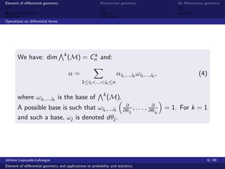
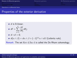
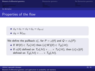
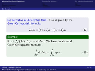
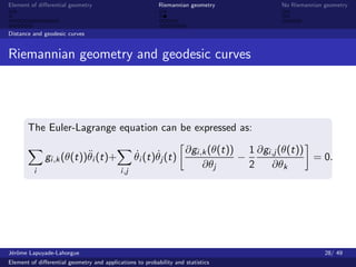
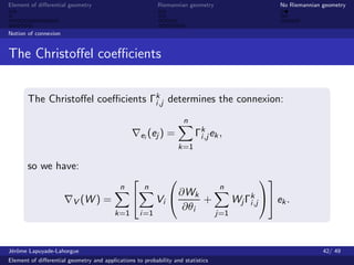
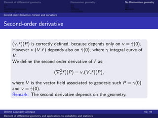
Operations on differential forms
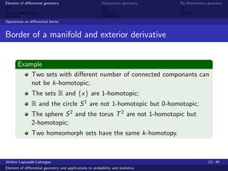
Border of a manifold and exterior derivative
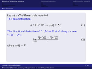
Definition
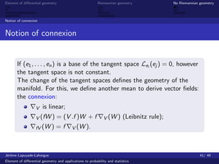
Let f and g two functions from E to F , f and g are k-homotopic
if there exists an application:
H : [0, 1]k × E → F , with [0, 1]0 = {0, 1} . (8)
such (u1 , . . . , uk ) → H(u1 , . . . , uk , x) continuous,
H(0, . . . , 0, x) = f (x) and H(1, . . . , 1, x) = g (x).
Two topological spaces E and F has the same k-homotopy if there
exists two functions f : E → F and g : F → E such g ◦ f and f ◦ g
are k-homotopic to the respective identity functions.
J´rˆme Lapuyade-Lahorgue
eo 11/ 49
Element of differential geometry and applications to probability and statistics

14. Element of differential geometry Riemannian geometry No Riemannian geometry
Operations on differential forms
Border of a manifold and exterior derivative
Example
Two sets with different number of connected componants can
not be k-homotopic;
The sets R and {x} are 1-homotopic;
R and the circle S 1 are not 1-homotopic but 0-homotopic;
The sphere S 2 and the torus T 2 are not 1-homotopic but
2-homotopic;
Two homeomorph sets have the same k-homotopy.
J´rˆme Lapuyade-Lahorgue
eo 12/ 49
Element of differential geometry and applications to probability and statistics

15. Element of differential geometry Riemannian geometry No Riemannian geometry
Operations on differential forms
Border of a manifold and exterior derivative
Definition
The border application is an application δ which associates to a
n-dimensional connexe manifold M:
If the manifold has the same n-homotopy than S n , δM = ∅;
If the manifold is homeomorph to the hypercube or an
half-space of Rn , δM is the image of the set of faces or the
delimitation of the half-space by the homeomorphism;
In other cases, the manifold has a hole, the border is the
union of the border of the manifold completed without the
hole and the border of the hole.
J´rˆme Lapuyade-Lahorgue
eo 13/ 49
Element of differential geometry and applications to probability and statistics

16. Element of differential geometry Riemannian geometry No Riemannian geometry
Operations on differential forms
Border of a manifold and exterior derivative
We have the following properties:
δM is either empty or dim δM = dim M − 1;
δδM = ∅;
If M is a star-shaped open set, then δM = ∅ implies that M
is a border;
The set Kerδ/Imδ is called De Rham homology.
J´rˆme Lapuyade-Lahorgue
eo 14/ 49
Element of differential geometry and applications to probability and statistics

17. Element of differential geometry Riemannian geometry No Riemannian geometry
Operations on differential forms
Border of a manifold and exterior derivative
The exterior derivative is an application d such
k
d (M) ⊂ k+1 (M) such that for any S ⊂ M,
k
k + 1-dimensional sub-manifold and for any α ∈ (M):
dα = α(Green-Stockes formula) (9)
S δS
There exists a unique linear d such (9) holds and:
n
∂f
df = dθj ;
∂θj
j=1
d(f α) = df ∧ α + fdα (Leibnitz rule).
J´rˆme Lapuyade-Lahorgue
eo 15/ 49
Element of differential geometry and applications to probability and statistics

18. Element of differential geometry Riemannian geometry No Riemannian geometry
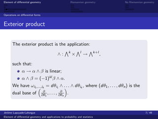
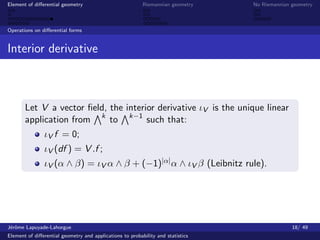
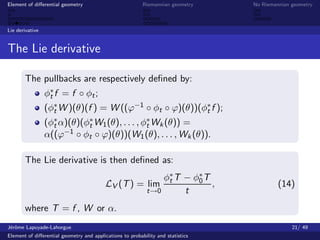
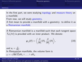
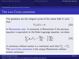
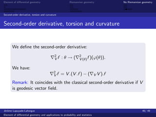
Operations on differential forms
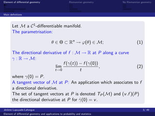
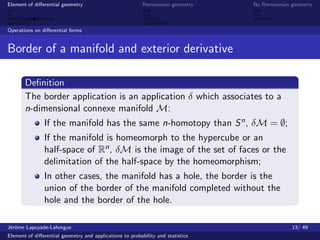
Orientation of the border
Let V = ϕ([0, 1]n ) a n-dimensional sub-manifold such δV = ∅ and
consider:
α = fdθ1 ∧ . . . ∧ θj−1 ∧ θj+1 ∧ . . . ∧ θn (10)
We have:
α = j [f (θj = 1) − f (θj = 0)] dθ1 . . . dθj−1 dθj+1 . . . dθn
δV [0,1]n−1
∂f
= j dθ1 . . . dθn
[0,1]n ∂θj
= j (−1)j−1 dα. (11)
V
So j = (−1)j−1 .
J´rˆme Lapuyade-Lahorgue
eo 16/ 49
Element of differential geometry and applications to probability and statistics

19. Element of differential geometry Riemannian geometry No Riemannian geometry
Operations on differential forms
Properties of the exterior derivative
d is R-linear;
n
∂f
df = dθj ;
∂θj
j=1
d ◦ d = 0;
d(α ∧ β) = dα ∧ β + (−1)|α| α ∧ dβ (Leibnitz rule).
Remark: The set Ker d/Im d is called the De Rham cohomology.
J´rˆme Lapuyade-Lahorgue
eo 17/ 49
Element of differential geometry and applications to probability and statistics

20. Element of differential geometry Riemannian geometry No Riemannian geometry
Operations on differential forms
Interior derivative
Let V a vector field, the interior derivative ιV is the unique linear
application from k to k−1 such that:
ιV f = 0;
ιV (df ) = V .f ;
ιV (α ∧ β) = ιV α ∧ β + (−1)|α| α ∧ ιV β (Leibnitz rule).
J´rˆme Lapuyade-Lahorgue
eo 18/ 49
Element of differential geometry and applications to probability and statistics

21. Element of differential geometry Riemannian geometry No Riemannian geometry
Lie derivative
Integral curves and flows
Let V be a vector field. An integral curve t → θ(t) with origine
P = ϕ(θ(0)) is a solution of:
˙
V (θ(t)) = θ(t), (12)
with:
n
˙
θ= ˙ ∂ .
θj (13)
∂θj
j=1
The flow (φt )t∈R of V is a set of applications φt which associates
to P ∈ M the point Q = ϕ(θ(t)), where θ is the integral curve
with origine P.
J´rˆme Lapuyade-Lahorgue
eo 19/ 49
Element of differential geometry and applications to probability and statistics

22. Element of differential geometry Riemannian geometry No Riemannian geometry
Lie derivative
Properties of the flow
φs ◦ φt = φt ◦ φs = φs+t ;
φ0 = IdM .
J´rˆme Lapuyade-Lahorgue
eo 20/ 49
Element of differential geometry and applications to probability and statistics

23. Element of differential geometry Riemannian geometry No Riemannian geometry
Lie derivative
Properties of the flow
φs ◦ φt = φt ◦ φs = φs+t ;
φ0 = IdM .
We define the pullback φ∗ , for P = ϕ(θ) and Q = φt (P):
t
If W (θ) ∈ TP (M) then (φ∗ W )(θ) ∈ TQ (M);
t
If α(θ) defined on TP (M) × . . . × TP (M), then (φ∗ α)(θ)
t
defined on TQ (M) × . . . × TQ (M).
J´rˆme Lapuyade-Lahorgue
eo 20/ 49
Element of differential geometry and applications to probability and statistics

24. Element of differential geometry Riemannian geometry No Riemannian geometry
Lie derivative
The Lie derivative
The pullbacks are respectively defined by:
φ∗ f = f ◦ φt ;
t
(φ∗ W )(θ)(f ) = W ((ϕ−1 ◦ φt ◦ ϕ)(θ))(φ∗ f );
t t
(φ∗ α)(θ)(φ∗ W1 (θ), . . . , φ∗ Wk (θ)) =
t t t
α((ϕ−1 ◦ φt ◦ ϕ)(θ))(W1 (θ), . . . , Wk (θ)).
The Lie derivative is then defined as:
φ∗ T − φ0 T
t
∗
LV (T ) = lim , (14)
t→0 t
where T = f , W or α.
J´rˆme Lapuyade-Lahorgue
eo 21/ 49
Element of differential geometry and applications to probability and statistics

25. Element of differential geometry Riemannian geometry No Riemannian geometry
Lie derivative
Properties of the Lie derivative
The Lie derivative satisfies:
T → LV T is linear;
LV (f ) = V .f : extends the directional derivative;
LV (fW ) = (V .f )W + f LV (W ): Leibnitz rule for vector fields;
LV (W .f ) = LV (W ).f + W .LV (f ): composition of
directional derivative;
LV (α ∧ β) = LV (α) ∧ β + α ∧ LV (β): Leibnitz rule for
differential form.
J´rˆme Lapuyade-Lahorgue
eo 22/ 49
Element of differential geometry and applications to probability and statistics

26. Element of differential geometry Riemannian geometry No Riemannian geometry
Lie derivative
Lie derivative of vector field: LV (W ) is the unique vector field
such that:
LV (W ).f = V .(W .f ) − W .(V .f ). (15)
Proof.
V .(W .f ) = LV (W .f ) because W .f is a function,
= LV (W ).f + W .LV (f ),
= LV (W ).f + W .(V .f ). (16)
J´rˆme Lapuyade-Lahorgue
eo 23/ 49
Element of differential geometry and applications to probability and statistics

27. Element of differential geometry Riemannian geometry No Riemannian geometry
Lie derivative
Lie derivative of differential form: LV α is given by the
Green-Ostrogradski formula:
LV α = (d ◦ ιV )α + (ιV ◦ d)α. (17)
Example
If ω ∈ n (M), LV ω = divV ω. We have the classical
Green-Ostrogradski formula:
divV ω = ιV ω. (18)
V δV
J´rˆme Lapuyade-Lahorgue
eo 24/ 49
Element of differential geometry and applications to probability and statistics

28. Element of differential geometry Riemannian geometry No Riemannian geometry
Definitions
In the first part, we were studying topology and measure theory on
a manifold.
From now, we will study geometry.
A first mean to provide a manifold with a geometry: to define it as
a Riemannian manifold.
A Riemannian manifold is a manifold such that each tangent space
TP (M) is provided with an inner product. We denote:
∂ ∂
gi ,j (θ) = (θ), (θ) , (19)
∂θi ∂θj
∂
and ei = ∂θi .
In Riemannian manifolds, the volume form is
√
ω = det G dθ1 ∧ . . . ∧ dθn .
J´rˆme Lapuyade-Lahorgue
eo 25/ 49
Element of differential geometry and applications to probability and statistics

29. Element of differential geometry Riemannian geometry No Riemannian geometry
Definitions
Example (The sphere S 2 )
A parametrisation and the associated base are:
 
 x = sin(θ) cos(ϕ)  eθ = cos(θ) cos(ϕ)ex + cos(θ) sin(ϕ)ey
y = sin(θ) sin(ϕ) − sin(θ)ez
z = cos(θ) eϕ = − sin(θ) sin(ϕ)ex + sin(θ) cos(ϕ)ey
 
If the inner product is inheritated from R3 then:
1 0
G= , (20)
0 sin2 θ
and the volume form is ω = sin θdθ ∧ dϕ.
J´rˆme Lapuyade-Lahorgue
eo 26/ 49
Element of differential geometry and applications to probability and statistics

30. Element of differential geometry Riemannian geometry No Riemannian geometry
Distance and geodesic curves
Riemannian geometry and geodesic curves
The distance between two points P = ϕ(θ (1) ) and Q = ϕ(θ (2) ) is
the minimum of:
t (2)
˙ ˙
gi ,j (θ(t))θi (t)θj (t)dt, (21)
t (1) i ,j
where t → θ(t) describes the set of curves of M.
˙ ˙ ˙
Let us denote L(θ, θ) = i ,j gi ,j (θ)θi θj , the minimum is reached
for t → θ(t), called geodesic curve, solution of:
∂L ˙ d ∂L ˙
(θ(t), θ(t)) − (θ(t), θ(t)) = 0. (22)
∂θk dt ˙
∂ θk
J´rˆme Lapuyade-Lahorgue
eo 27/ 49
Element of differential geometry and applications to probability and statistics

31. Element of differential geometry Riemannian geometry No Riemannian geometry
Distance and geodesic curves
Riemannian geometry and geodesic curves
The Euler-Lagrange equation can be expressed as:
¨ ˙ ˙ ∂gi ,k (θ(t)) 1 ∂gi ,j (θ(t))
gi ,k (θ(t))θi (t)+ θi (t)θj (t) − = 0.
∂θj 2 ∂θk
i i ,j
J´rˆme Lapuyade-Lahorgue
eo 28/ 49
Element of differential geometry and applications to probability and statistics

32. Element of differential geometry Riemannian geometry No Riemannian geometry
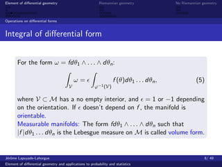
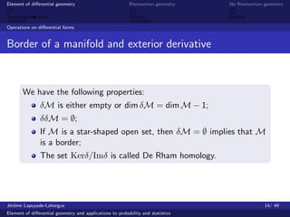
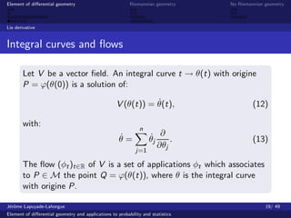
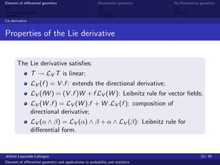
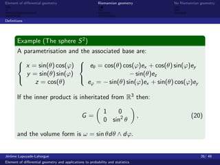
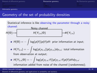
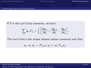
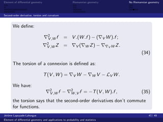
Information geometry
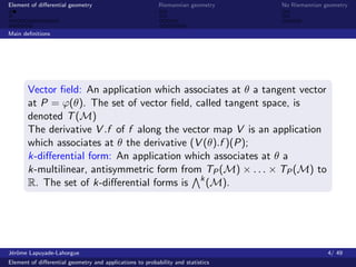
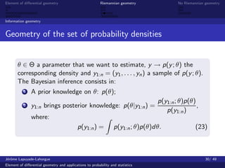
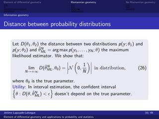
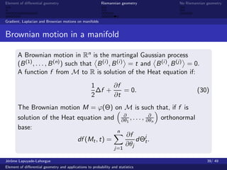
Geometry of the set of probability densities
We study parameterized set of probability distribution.
At each θ ∈ Θ ⊂ Rk , we associate a probability density
y → p(y ; θ):
b
p(y ; θ)dy = 1 and Pθ (Y ∈ [a, b]) = p(y ; θ)dy ;
a
For each fixed y , θ → p(y ; θ) is differentiable.
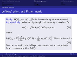
The Riemannian metric is chosen in order to the volume form is
the prior distribution such that an infinite sample of p(y ; θ)
provides the maximum of information.
J´rˆme Lapuyade-Lahorgue
eo 29/ 49
Element of differential geometry and applications to probability and statistics

33. Element of differential geometry Riemannian geometry No Riemannian geometry
Information geometry
Geometry of the set of probability densities
θ ∈ Θ a parameter that we want to estimate, y → p(y ; θ) the
corresponding density and y1:n = (y1 , . . . , yn ) a sample of p(y ; θ).
The Bayesian inference consists in:
1 A prior knowledge on θ: p(θ);
p(y1:n ; θ)p(θ)
2 y1:n brings posterior knowledge: p(θ|y1:n ) = ,
p(y1:n )
where:
p(y1:n ) = p(y1:n ; θ)p(θ)dθ. (23)
J´rˆme Lapuyade-Lahorgue
eo 30/ 49
Element of differential geometry and applications to probability and statistics

34. Element of differential geometry Riemannian geometry No Riemannian geometry
Information geometry
Geometry of the set of probability densities
Statistical inference is like observing the parameter through a noisy
channel:
Noisy channel
H(Θ) H(Y1:n |Θ) H(Y1:n )
H(Θ) = − log(p(θ))p(θ)dθ: prior information at input;
H(Y1:n ) = − log(p(y1:n ))p(y1:n )dy1:n : total information
from observation at output;
H(Y1:n |Θ) = − log(p(y1:n ; θ))p(y1:n ; θ)p(θ)dθdy1:n :
information added from noise of the channel (randomness);
J´rˆme Lapuyade-Lahorgue
eo 31/ 49
Element of differential geometry and applications to probability and statistics

35. Element of differential geometry Riemannian geometry No Riemannian geometry
Information geometry
Jeffreys’ priors and Fisher metric
Finally: H(Y1:n ) − H(Y1:n |Θ) is the remaining information on θ.
Asymptotically: When N big enough, this quantity is maximal for:
p(θ) ∝ det IY (θ) Jeffreys prior. (24)
where:
∂ ∂
IY (θ)i ,j = E log p(Y ; θ) × log p(Y ; θ) Fisher information.
∂θi ∂θj
(25)
One can show that the Jeffreys prior corresponds to the volume
form, consequently G = IY (θ).
J´rˆme Lapuyade-Lahorgue
eo 32/ 49
Element of differential geometry and applications to probability and statistics

36. Element of differential geometry Riemannian geometry No Riemannian geometry
Information geometry
Distance between probability distributions
Let D(θ1 , θ2 ) the distance between two distributions p(y ; θ1 ) and
ˆN
p(y ; θ2 ) and θML = arg max p(y1 , . . . , yN ; θ) the maximum
likelihood estimator. We show that:
ˆN 1
lim D(θML , θ0 ) = N 0, in distribution, (26)
N→+∞ N
where θ0 is the true parameter.
Utility: In interval estimation, the confident interval
ˆN
θ : D(θ, θML) < doesn’t depend on the true parameter.
J´rˆme Lapuyade-Lahorgue
eo 33/ 49
Element of differential geometry and applications to probability and statistics

37. Element of differential geometry Riemannian geometry No Riemannian geometry
Gradient, Laplacian and Brownian motions on manifolds
The gradient and Laplace-Beltrami operator
Let f be a function from M to R, there exists a unique vector
field, called gradient of f , denoted gradf such that:
gradf , V = df (V ), (27)
for all vector fields V .
The Laplace-Beltrami operator of f is defined as:
∆f = divgradf . (28)
J´rˆme Lapuyade-Lahorgue
eo 34/ 49
Element of differential geometry and applications to probability and statistics

38. Element of differential geometry Riemannian geometry No Riemannian geometry
Gradient, Laplacian and Brownian motions on manifolds
Denote g i ,j the coefficients of G −1 , we have:
∂f ∂f
gradf = G −1 e1 + . . . + en ;
∂θ1 ∂θ1
 
n n
∂Vj 1 ∂gk,i 
divV =  + Vj g i ,k ;
∂θj 2 ∂θj
j=1 i ,k=1
n n
∂2f ∂g i ,j ∂f
∆f = g i ,j +
∂θi ∂θj ∂θj ∂θi
j=1 i =1
 
n n
1 ∂f  ∂gk,i 
+ g l,j g i ,k .
2 ∂θl ∂θj
l=1 i ,k=1
J´rˆme Lapuyade-Lahorgue
eo 35/ 49
Element of differential geometry and applications to probability and statistics

39. Element of differential geometry Riemannian geometry No Riemannian geometry
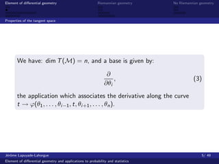
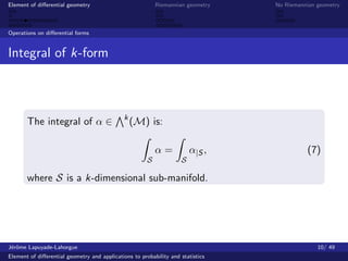
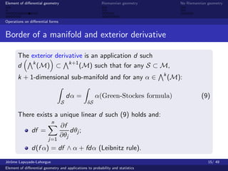
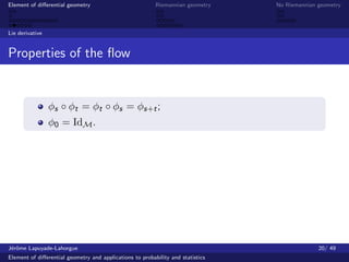
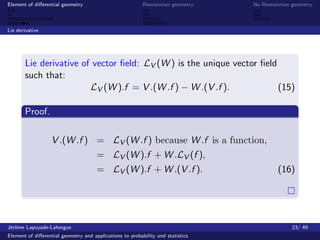
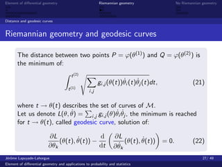
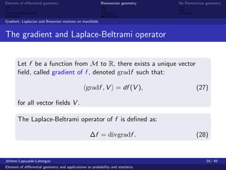
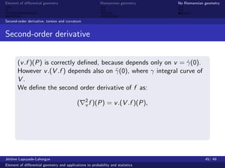
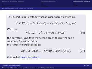
Gradient, Laplacian and Brownian motions on manifolds
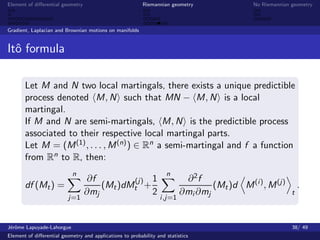
Martingals, local martingals and semi-martingals
Let (Ω, A, P) a probability space.
A continuous time process (Mt ) is a martingal if
E [Mt |σ((Mu )u≤s )] = Ms for any s ≤ t;
A continuous time process (Mt ) is a local martingal if there
exists an increasing sequence of stopping times (Tn ) such that
the processes (Mt∧Tn ) are martingals;
A predictible process (At ) is a process such that for any
ω ∈ Ω, there exists a Radon measure µ(ω) such that
At (ω) − As (ω) = µ(ω) (]s, t]);
A semi-martingal is the sum of a local martingal and a
predictible process.
J´rˆme Lapuyade-Lahorgue
eo 36/ 49
Element of differential geometry and applications to probability and statistics

40. Element of differential geometry Riemannian geometry No Riemannian geometry
Gradient, Laplacian and Brownian motions on manifolds
Stochastic integral and differential forms
If M and N are two semi-martingals, we define the Itˆ integral:
o
t n−1
2
f (Ms )dNs =L lim f (Mtk )(Ntk+1 − Ntk );
0 n→+∞
k=0
(29)
t
Pt = 0 f (Ms )dNs will be denoted dPt = f (Ms )dNs .
J´rˆme Lapuyade-Lahorgue
eo 37/ 49
Element of differential geometry and applications to probability and statistics

41. Element of differential geometry Riemannian geometry No Riemannian geometry
Gradient, Laplacian and Brownian motions on manifolds
Itˆ formula
o
Let M and N two local martingals, there exists a unique predictible
process denoted M, N such that MN − M, N is a local
martingal.
If M and N are semi-martingals, M, N is the predictible process
associated to their respective local martingal parts.
Let M = (M (1) , . . . , M (n) ) ∈ Rn a semi-martingal and f a function
from Rn to R, then:
n n
∂f (j) 1 ∂2f
df (Mt ) = (Mt )dMt + (Mt )d M (i ) , M (j) .
∂mj 2 ∂mi ∂mj t
j=1 i ,j=1
J´rˆme Lapuyade-Lahorgue
eo 38/ 49
Element of differential geometry and applications to probability and statistics

42. Element of differential geometry Riemannian geometry No Riemannian geometry
Gradient, Laplacian and Brownian motions on manifolds
Brownian motion in a manifold
A Brownian motion in Rn is the martingal Gaussian process
(B (1) , . . . , B (n) ) such that B (i ) , B (i ) = t and B (i ) , B (j) = 0.
A function f from M to R is solution of the Heat equation if:
1 ∂f
∆f + = 0. (30)
2 ∂t
The Brownian motion M = ϕ(Θ) on M is such that, if f is
∂ ∂
solution of the Heat equation and ∂θ1 , . . . , ∂θn orthonormal
base:
n
∂f
df (Mt , t) = dΘj . t
∂θj
j=1
J´rˆme Lapuyade-Lahorgue
eo 39/ 49
Element of differential geometry and applications to probability and statistics

43. Element of differential geometry Riemannian geometry No Riemannian geometry
Gradient, Laplacian and Brownian motions on manifolds
Expression of the Brownian motion
n
∂ ∂2
If ∆ = ai + bi ,j , then:
∂θi ∂θi ∂θj
i =1 i ,j
k
(i ) ai (i ) (l)
dΘt = dt + αl dBt , (31)
2
l=1
where B (l) is Brownian motion on R and:
 (1) (1)   (1) (k)   
α1 . . . αk α1 . . . α1 b1,1 . . . b1,k
 . . . × . . . = . . . .
 . . .
. .   .
. . .
. .   .
. . .
. . 
.
(k) (k) (1) (k) bk,1 . . . bk,k
α1 . . . αk αk . . . αk
J´rˆme Lapuyade-Lahorgue
eo 40/ 49
Element of differential geometry and applications to probability and statistics

44. Element of differential geometry Riemannian geometry No Riemannian geometry
Notion of connexion
Notion of connexion
If (e1 , . . . , en ) is a base of the tangent space Lei (ej ) = 0, however
the tangent space is not constant.
The change of the tangent spaces defines the geometry of the
manifold. For this, we define another mean to derive vector fields:
the connexion:
V is linear;
V (fW ) = (V .f )W + f V (W ) (Leibnitz rule);
fV (W ) =f V (W ).
J´rˆme Lapuyade-Lahorgue
eo 41/ 49
Element of differential geometry and applications to probability and statistics

45. Element of differential geometry Riemannian geometry No Riemannian geometry
Notion of connexion
The Christoffel coefficients
The Christoffel coefficients Γk,j determines the connexion:
i
n
ei (ej ) = Γik,j ek ,
k=1
so we have:
  
n n n
∂Wk
V (W ) =  Vi  + Wj Γk,j  ek .
i
∂θi
k=1 i =1 j=1
J´rˆme Lapuyade-Lahorgue
eo 42/ 49
Element of differential geometry and applications to probability and statistics

46. Element of differential geometry Riemannian geometry No Riemannian geometry
The Riemannian case and Levi-Civita connexion
The Levi-Civita connexion
The geodesics are the integral curves of the vector field V such
that:
V (V ) = 0. (32)
In Riemannian case: A connexion is Riemannian if the previous
equation is equivalent to the Euler-Lagrange equation, we show:
∂gl,k 1 ∂gl,j
gi ,k Γil,j = − . (33)
∂θj 2 ∂θk
k
A connexion without torsion is a connexion such that Γk,j = Γk .
i j,i
The Levi-Civita connexion is the unique Riemannian without
torsion connexion.
J´rˆme Lapuyade-Lahorgue
eo 43/ 49
Element of differential geometry and applications to probability and statistics

47. Element of differential geometry Riemannian geometry No Riemannian geometry
The Riemannian case and Levi-Civita connexion
If is the Levi-Civita connexion, we have:
i 1 ∂gl,k ∂gj,k ∂gl,j
gi ,k Γl,j = + − .
2 ∂θj ∂θl ∂θk
k
The Levi-Civita is the unique without torsion connexion such that:
ek . ei , ej = ek ei , ej + ei , ek ej .
J´rˆme Lapuyade-Lahorgue
eo 44/ 49
Element of differential geometry and applications to probability and statistics

48. Element of differential geometry Riemannian geometry No Riemannian geometry
Second-order derivative, torsion and curvature
Second-order derivative
(v .f )(P) is correctly defined, because depends only on v = γ(0).
˙
However v .(V .f ) depends also on γ (0), where γ integral curve of
¨
V.
We define the second order derivative of f as:
2
( v f )(P) = v .(V .f )(P),
J´rˆme Lapuyade-Lahorgue
eo 45/ 49
Element of differential geometry and applications to probability and statistics

49. Element of differential geometry Riemannian geometry No Riemannian geometry
Second-order derivative, torsion and curvature
Second-order derivative
(v .f )(P) is correctly defined, because depends only on v = γ(0).
˙
However v .(V .f ) depends also on γ (0), where γ integral curve of
¨
V.
We define the second order derivative of f as:
2
( v f )(P) = v .(V .f )(P),
where V is the vector field associated to geodesic such P = γ(0)
and v = γ(0).
˙
Remark: The second derivative depends on the geometry.
J´rˆme Lapuyade-Lahorgue
eo 45/ 49
Element of differential geometry and applications to probability and statistics

50. Element of differential geometry Riemannian geometry No Riemannian geometry
Second-order derivative, torsion and curvature
Second-order derivative, torsion and curvature
We define the second-order derivative:
2 2
Vf :θ→( V (θ) f )(ϕ(θ)).
We have:
2
Vf = V .(V .f ) − ( V V ).f
Remark: It coincides with the classical second-order derivative if V
is geodesic vector field.
J´rˆme Lapuyade-Lahorgue
eo 46/ 49
Element of differential geometry and applications to probability and statistics

51. Element of differential geometry Riemannian geometry No Riemannian geometry
Second-order derivative, torsion and curvature
We define:
2
V ,W f = V .(W .f ) − ( V W ).f ;
2
V ,W Z = V( W Z) − VW
Z.
(34)
The torsion of a connexion is defined as:
T (V , W ) = VW − WV − LV W .
We have:
2 2
V ,W f − W ,V f = −T (V , W ).f , (35)
the torsion says that the second-order derivatives don’t commute
for functions.
J´rˆme Lapuyade-Lahorgue
eo 47/ 49
Element of differential geometry and applications to probability and statistics

52. Element of differential geometry Riemannian geometry No Riemannian geometry
Second-order derivative, torsion and curvature
The curvature of a without torsion connexion is defined as:
R(V , W , Z ) = V( W Z) − W( V Z) − LV W Z .
We have:
2 2
V ,W Z − W ,V Z = R(V , W , Z ), (36)
the curvature says that the second-order derivatives don’t
commute for vector fields.
In a three dimensional space:
R(V , W , Z ).U = −K Vol(V , W )Vol(Z , U), (37)
K is called Gauss curvature.
J´rˆme Lapuyade-Lahorgue
eo 48/ 49
Element of differential geometry and applications to probability and statistics

53. Element of differential geometry Riemannian geometry No Riemannian geometry
Second-order derivative, torsion and curvature
No riemannian set of probability distributions
The study of no Riemannian or information geometry with torsion
has been by S. I. Amari and H. Nagaoka in Methods of Information
Geometry
J´rˆme Lapuyade-Lahorgue
eo 49/ 49
Element of differential geometry and applications to probability and statistics