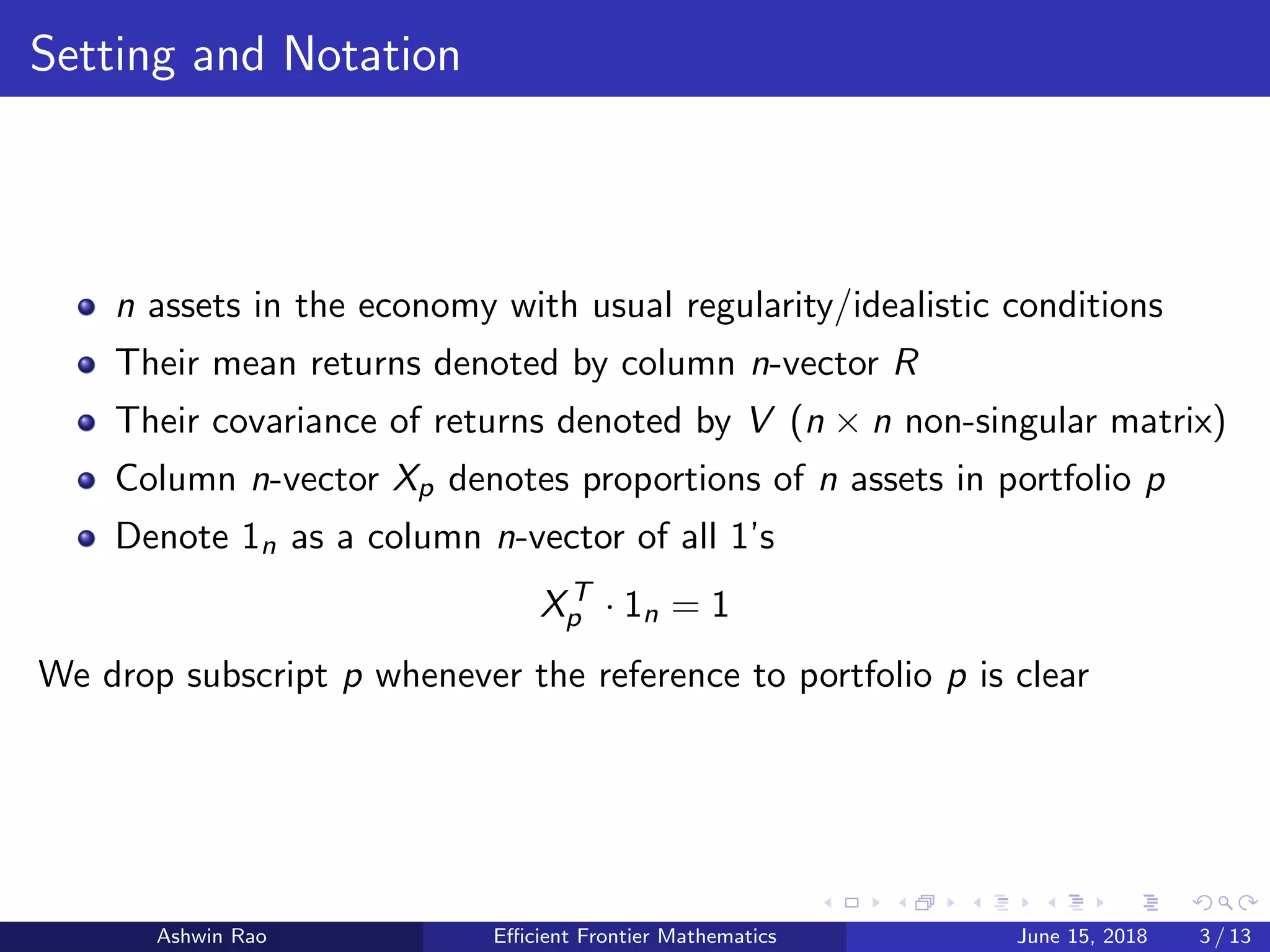
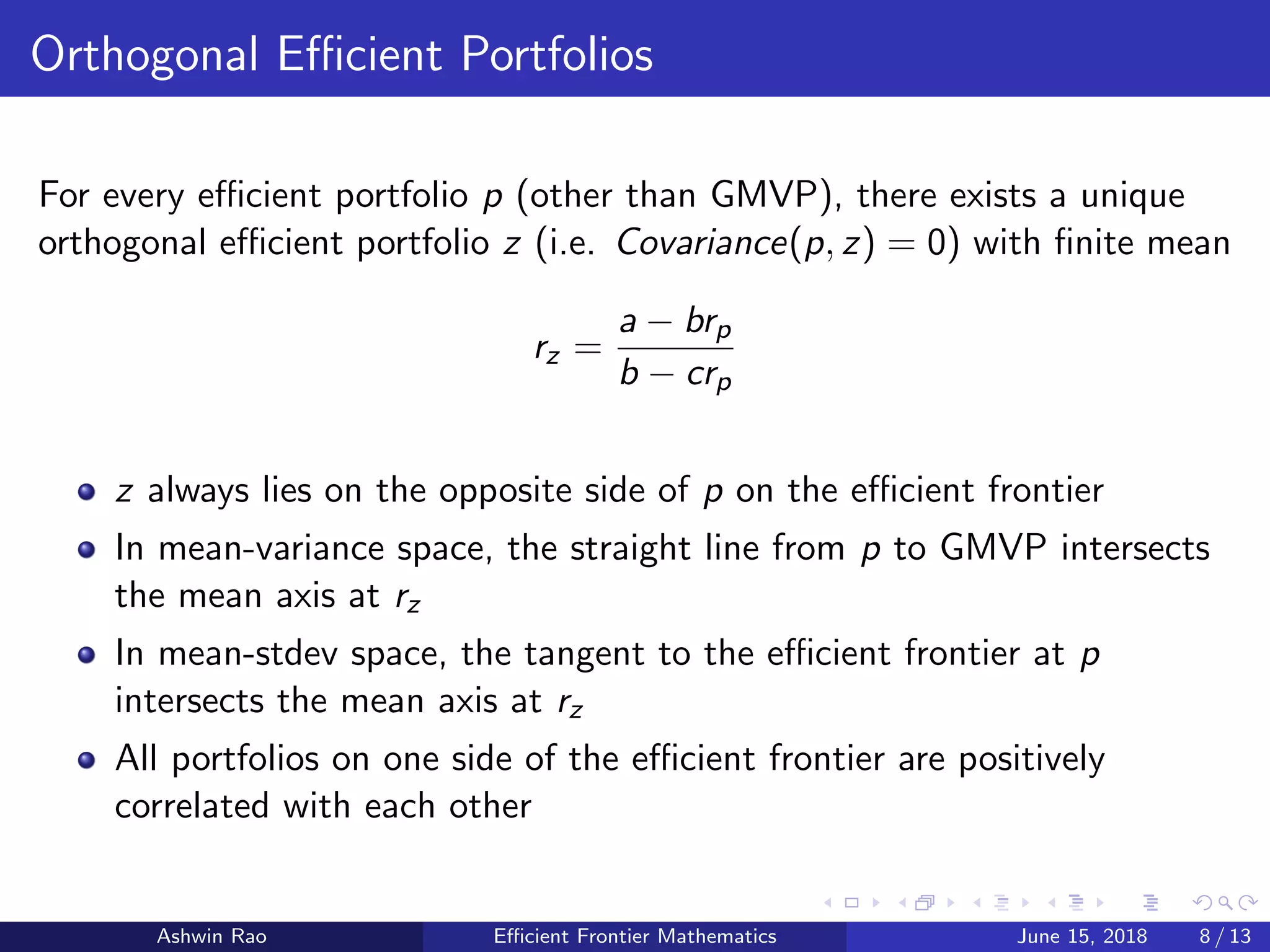
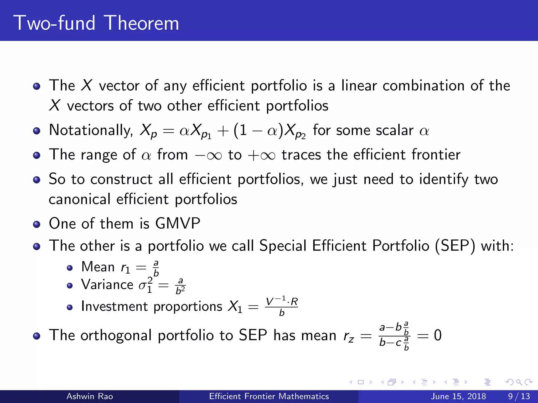
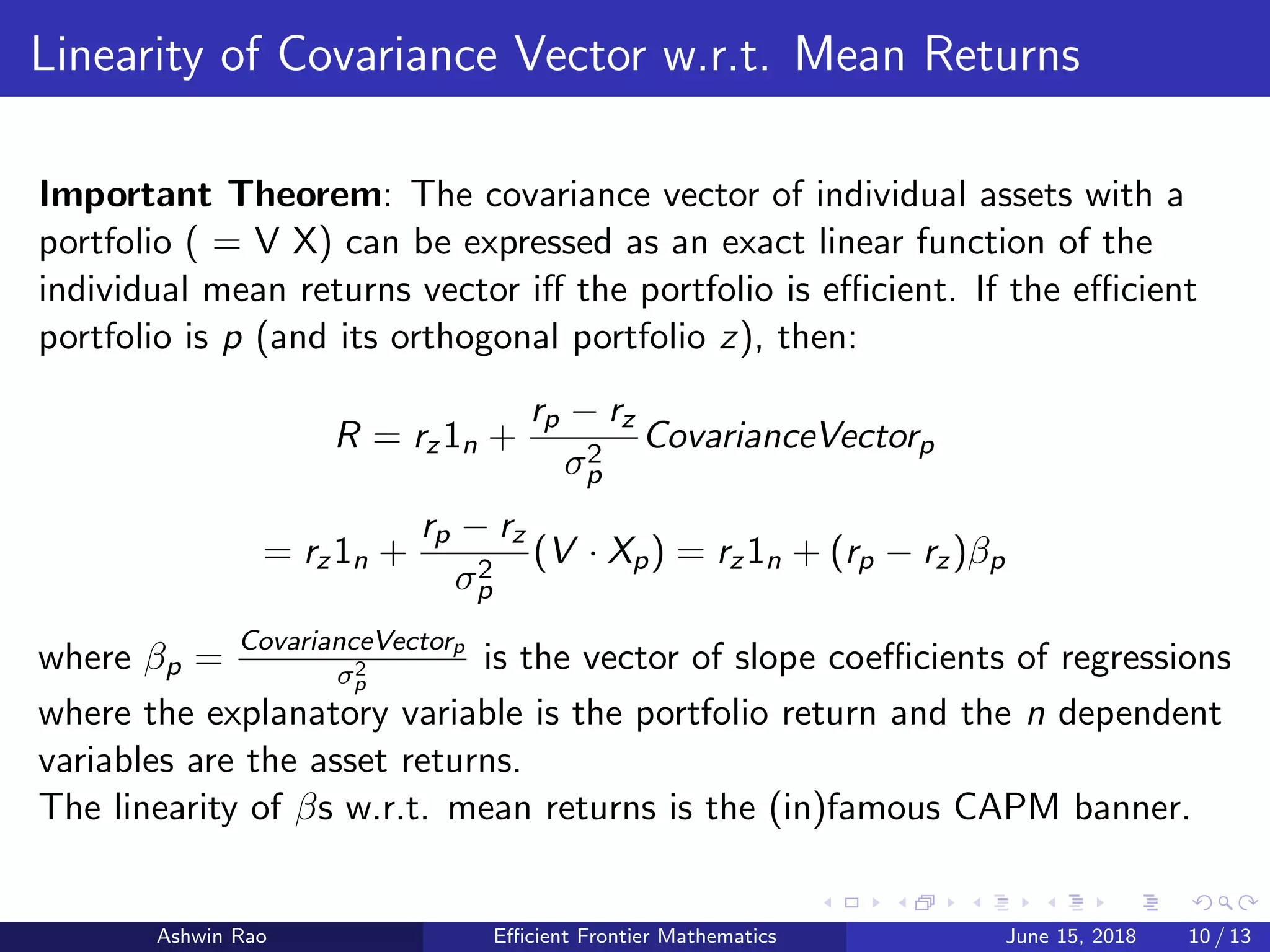
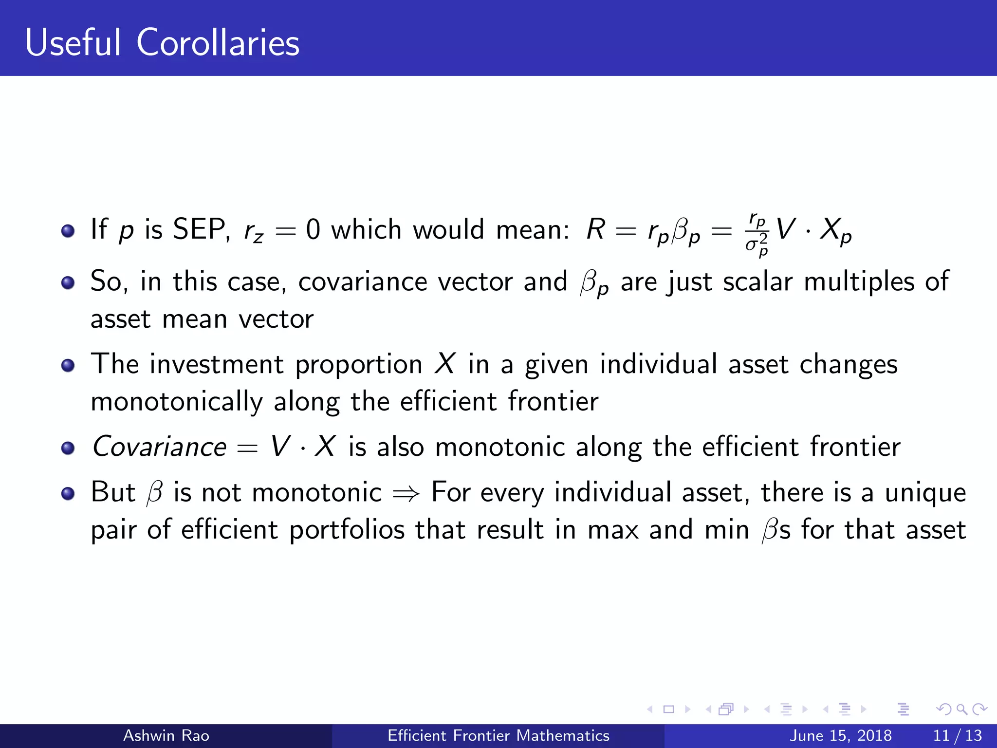
A Quick/Terse Intro to Efficient Frontier Mathematics
Ashwin Rao
June 15, 2018
Ashwin Rao Efficient Frontier Mathematics June 15, 2018 1 / 13
Overview
1 Setting and Notation
2 Derivation of Efficient Frontier Curve
3 Interesting Efficient Portfolios
4 Linearity of Covariance Vector w.r.t. Mean Returns (a.k.a. CAPM)
5 Efficient Set with a Risk-Free Asset
Ashwin Rao Efficient Frontier Mathematics June 15, 2018 2 / 13
Setting and Notation
n assets in the economy with usual regularity/idealistic conditions
Their mean returns denoted by column n-vector R
Their covariance of returns denoted by V (n × n non-singular matrix)
Column n-vector Xp denotes proportions of n assets in portfolio p
Denote 1n as a column n-vector of all 1’s
XT
p · 1n = 1
We drop subscript p whenever the reference to portfolio p is clear
Ashwin Rao Efficient Frontier Mathematics June 15, 2018 3 / 13
Portfolio Returns
A single portfolio’s mean return is XT · R
A single portfolio’s variance of return is the quadratic form XT · V · X
Covariance between portfolios p and q is the bilinear form XT
p · V · Xq
Covariance of assets with a single portfolio is V · X (n-vector)
Ashwin Rao Efficient Frontier Mathematics June 15, 2018 4 / 13
Derivation of Efficient Frontier Curve
Efficient frontier is defined for a world with no risk-free assets
It is the set of portfolios with minimum variance of return for each
level of portfolio mean returns
So, minimize portfolio variance XT · Vp · X subject to constraints:
XT
· 1n = 1
XT
· R = rp
where rp is the mean return for efficient portfolio p.
Set up the Lagrangian and solve to express X in terms of R, V , rp
Substituting for X gives us the efficient frontier parabola:
σ2
p =
a − 2brp + cr2
p
ac − b2
where
a = RT
· V −1
· R, b = RT
· V −1
· 1n, c = 1T
n V −1
1n
Ashwin Rao Efficient Frontier Mathematics June 15, 2018 5 / 13
The Efficient Frontier with 16 assets
Ashwin Rao Efficient Frontier Mathematics June 15, 2018 6 / 13
Global Minimum Variance Portfolio (GMVP)
Global minimum variance portfolio (GMVP) is the tip of the curve
It has mean r0 = b
c
It has variance σ2
0 = 1
c
It has investment proportions X0 = V −1·1n
c
GMVP is positively correlated with all portfolios and assets
GMVP’s covariance with all assets and all portfolios is a constant σ2
0
(which is also equal to its own variance)
Ashwin Rao Efficient Frontier Mathematics June 15, 2018 7 / 13
Orthogonal Efficient Portfolios
For every efficient portfolio p (other than GMVP), there exists a unique
orthogonal efficient portfolio z (i.e. Covariance(p, z) = 0) with finite mean
rz =
a − brp
b − crp
z always lies on the opposite side of p on the efficient frontier
In mean-variance space, the straight line from p to GMVP intersects
the mean axis at rz
In mean-stdev space, the tangent to the efficient frontier at p
intersects the mean axis at rz
All portfolios on one side of the efficient frontier are positively
correlated with each other
Ashwin Rao Efficient Frontier Mathematics June 15, 2018 8 / 13
Two-fund Theorem
The X vector of any efficient portfolio is a linear combination of the
X vectors of two other efficient portfolios
Notationally, Xp = αXp1 + (1 − α)Xp2 for some scalar α
The range of α from −∞ to +∞ traces the efficient frontier
So to construct all efficient portfolios, we just need to identify two
canonical efficient portfolios
One of them is GMVP
The other is a portfolio we call Special Efficient Portfolio (SEP) with:
Mean r1 = a
b
Variance σ2
1 = a
b2
Investment proportions X1 = V −1
·R
b
The orthogonal portfolio to SEP has mean rz =
a−b a
b
b−c a
b
= 0
Ashwin Rao Efficient Frontier Mathematics June 15, 2018 9 / 13
Linearity of Covariance Vector w.r.t. Mean Returns
Important Theorem: The covariance vector of individual assets with a
portfolio ( = V X) can be expressed as an exact linear function of the
individual mean returns vector iff the portfolio is efficient. If the efficient
portfolio is p (and its orthogonal portfolio z), then:
R = rz1n +
rp − rz
σ2
p
CovarianceVectorp
= rz1n +
rp − rz
σ2
p
(V · Xp) = rz1n + (rp − rz)βp
where βp =
CovarianceVectorp
σ2
p
is the vector of slope coefficients of regressions
where the explanatory variable is the portfolio return and the n dependent
variables are the asset returns.
The linearity of βs w.r.t. mean returns is the (in)famous CAPM banner.
Ashwin Rao Efficient Frontier Mathematics June 15, 2018 10 / 13
Useful Corollaries
If p is SEP, rz = 0 which would mean: R = rpβp =
rp
σ2
p
V · Xp
So, in this case, covariance vector and βp are just scalar multiples of
asset mean vector
The investment proportion X in a given individual asset changes
monotonically along the efficient frontier
Covariance = V · X is also monotonic along the efficient frontier
But β is not monotonic ⇒ For every individual asset, there is a unique
pair of efficient portfolios that result in max and min βs for that asset
Ashwin Rao Efficient Frontier Mathematics June 15, 2018 11 / 13
Cross-Sectional Variance
The cross-sectional variance in βs (variance in βs across assets for a
fixed efficient portfolio) is zero when efficient portfolio is GMVP and
when efficient portfolio has infinite mean
The cross-sectional variance in βs is maximum for the two efficient
portfolios with means: r0 ± σ2
0 |A| where A is the 2 × 2 matrix
consisting of a, b, b, c
These two portfolios lie symmetrically on opposite sides of the efficient
frontier (their βs are equal and of opposite signs), and are the only
two orthogonal efficient portfolios with the same variance ( = 2σ2
0)
Ashwin Rao Efficient Frontier Mathematics June 15, 2018 12 / 13
Efficient Set with a Risk-Free Asset
If we have a risk-free asset with return rF , V is singular
First form the efficient frontier without the risk-free asset
The efficient set (with a risk-free asset) is the tangent to the efficient
frontier (without the risk-free asset) in mean-stdev space from (0, rF )
Let tangency point portfolio be T with return rT
If rF < r0, rT > rF
If rF > r0, rT < rF
All portfolios on this efficient set are perfectly correlated
Homework: How is T related to SEP?
Ashwin Rao Efficient Frontier Mathematics June 15, 2018 13 / 13

A Quick and Terse Introduction to Efficient Frontier Mathematics

  • 1.
    A Quick/Terse Introto Efficient Frontier Mathematics Ashwin Rao June 15, 2018 Ashwin Rao Efficient Frontier Mathematics June 15, 2018 1 / 13
  • 2.
    Overview 1 Setting andNotation 2 Derivation of Efficient Frontier Curve 3 Interesting Efficient Portfolios 4 Linearity of Covariance Vector w.r.t. Mean Returns (a.k.a. CAPM) 5 Efficient Set with a Risk-Free Asset Ashwin Rao Efficient Frontier Mathematics June 15, 2018 2 / 13
  • 3.
    Setting and Notation nassets in the economy with usual regularity/idealistic conditions Their mean returns denoted by column n-vector R Their covariance of returns denoted by V (n × n non-singular matrix) Column n-vector Xp denotes proportions of n assets in portfolio p Denote 1n as a column n-vector of all 1’s XT p · 1n = 1 We drop subscript p whenever the reference to portfolio p is clear Ashwin Rao Efficient Frontier Mathematics June 15, 2018 3 / 13
  • 4.
    Portfolio Returns A singleportfolio’s mean return is XT · R A single portfolio’s variance of return is the quadratic form XT · V · X Covariance between portfolios p and q is the bilinear form XT p · V · Xq Covariance of assets with a single portfolio is V · X (n-vector) Ashwin Rao Efficient Frontier Mathematics June 15, 2018 4 / 13
  • 5.
    Derivation of EfficientFrontier Curve Efficient frontier is defined for a world with no risk-free assets It is the set of portfolios with minimum variance of return for each level of portfolio mean returns So, minimize portfolio variance XT · Vp · X subject to constraints: XT · 1n = 1 XT · R = rp where rp is the mean return for efficient portfolio p. Set up the Lagrangian and solve to express X in terms of R, V , rp Substituting for X gives us the efficient frontier parabola: σ2 p = a − 2brp + cr2 p ac − b2 where a = RT · V −1 · R, b = RT · V −1 · 1n, c = 1T n V −1 1n Ashwin Rao Efficient Frontier Mathematics June 15, 2018 5 / 13
  • 6.
    The Efficient Frontierwith 16 assets Ashwin Rao Efficient Frontier Mathematics June 15, 2018 6 / 13
  • 7.
    Global Minimum VariancePortfolio (GMVP) Global minimum variance portfolio (GMVP) is the tip of the curve It has mean r0 = b c It has variance σ2 0 = 1 c It has investment proportions X0 = V −1·1n c GMVP is positively correlated with all portfolios and assets GMVP’s covariance with all assets and all portfolios is a constant σ2 0 (which is also equal to its own variance) Ashwin Rao Efficient Frontier Mathematics June 15, 2018 7 / 13
  • 8.
    Orthogonal Efficient Portfolios Forevery efficient portfolio p (other than GMVP), there exists a unique orthogonal efficient portfolio z (i.e. Covariance(p, z) = 0) with finite mean rz = a − brp b − crp z always lies on the opposite side of p on the efficient frontier In mean-variance space, the straight line from p to GMVP intersects the mean axis at rz In mean-stdev space, the tangent to the efficient frontier at p intersects the mean axis at rz All portfolios on one side of the efficient frontier are positively correlated with each other Ashwin Rao Efficient Frontier Mathematics June 15, 2018 8 / 13
  • 9.
    Two-fund Theorem The Xvector of any efficient portfolio is a linear combination of the X vectors of two other efficient portfolios Notationally, Xp = αXp1 + (1 − α)Xp2 for some scalar α The range of α from −∞ to +∞ traces the efficient frontier So to construct all efficient portfolios, we just need to identify two canonical efficient portfolios One of them is GMVP The other is a portfolio we call Special Efficient Portfolio (SEP) with: Mean r1 = a b Variance σ2 1 = a b2 Investment proportions X1 = V −1 ·R b The orthogonal portfolio to SEP has mean rz = a−b a b b−c a b = 0 Ashwin Rao Efficient Frontier Mathematics June 15, 2018 9 / 13
  • 10.
    Linearity of CovarianceVector w.r.t. Mean Returns Important Theorem: The covariance vector of individual assets with a portfolio ( = V X) can be expressed as an exact linear function of the individual mean returns vector iff the portfolio is efficient. If the efficient portfolio is p (and its orthogonal portfolio z), then: R = rz1n + rp − rz σ2 p CovarianceVectorp = rz1n + rp − rz σ2 p (V · Xp) = rz1n + (rp − rz)βp where βp = CovarianceVectorp σ2 p is the vector of slope coefficients of regressions where the explanatory variable is the portfolio return and the n dependent variables are the asset returns. The linearity of βs w.r.t. mean returns is the (in)famous CAPM banner. Ashwin Rao Efficient Frontier Mathematics June 15, 2018 10 / 13
  • 11.
    Useful Corollaries If pis SEP, rz = 0 which would mean: R = rpβp = rp σ2 p V · Xp So, in this case, covariance vector and βp are just scalar multiples of asset mean vector The investment proportion X in a given individual asset changes monotonically along the efficient frontier Covariance = V · X is also monotonic along the efficient frontier But β is not monotonic ⇒ For every individual asset, there is a unique pair of efficient portfolios that result in max and min βs for that asset Ashwin Rao Efficient Frontier Mathematics June 15, 2018 11 / 13
  • 12.
    Cross-Sectional Variance The cross-sectionalvariance in βs (variance in βs across assets for a fixed efficient portfolio) is zero when efficient portfolio is GMVP and when efficient portfolio has infinite mean The cross-sectional variance in βs is maximum for the two efficient portfolios with means: r0 ± σ2 0 |A| where A is the 2 × 2 matrix consisting of a, b, b, c These two portfolios lie symmetrically on opposite sides of the efficient frontier (their βs are equal and of opposite signs), and are the only two orthogonal efficient portfolios with the same variance ( = 2σ2 0) Ashwin Rao Efficient Frontier Mathematics June 15, 2018 12 / 13
  • 13.
    Efficient Set witha Risk-Free Asset If we have a risk-free asset with return rF , V is singular First form the efficient frontier without the risk-free asset The efficient set (with a risk-free asset) is the tangent to the efficient frontier (without the risk-free asset) in mean-stdev space from (0, rF ) Let tangency point portfolio be T with return rT If rF < r0, rT > rF If rF > r0, rT < rF All portfolios on this efficient set are perfectly correlated Homework: How is T related to SEP? Ashwin Rao Efficient Frontier Mathematics June 15, 2018 13 / 13