Download as PDF, PPTX
![Discretised Hamiltonian
Girolami and Calderhead reproduce Hamiltonian equations within
the simulation domain by discretisation via the generalised leapfrog
(!) generator,
[Subliminal French bashing?!]
Christian P. Robert About discretising Hamiltonians](https://image.slidesharecdn.com/rs1013-coms-101013153858-phpapp02/75/RSS-discussion-of-Girolami-and-Calderhead-October-13-2010-3-2048.jpg)
![Discretised Hamiltonian
Girolami and Calderhead reproduce Hamiltonian equations within
the simulation domain by discretisation via the generalised leapfrog
(!) generator,
but...
invariance and stability properties of the [background] continuous
time process the method do not carry to the discretised version of
the process [e.g., Langevin]
Christian P. Robert About discretising Hamiltonians](https://image.slidesharecdn.com/rs1013-coms-101013153858-phpapp02/75/RSS-discussion-of-Girolami-and-Calderhead-October-13-2010-5-2048.jpg)
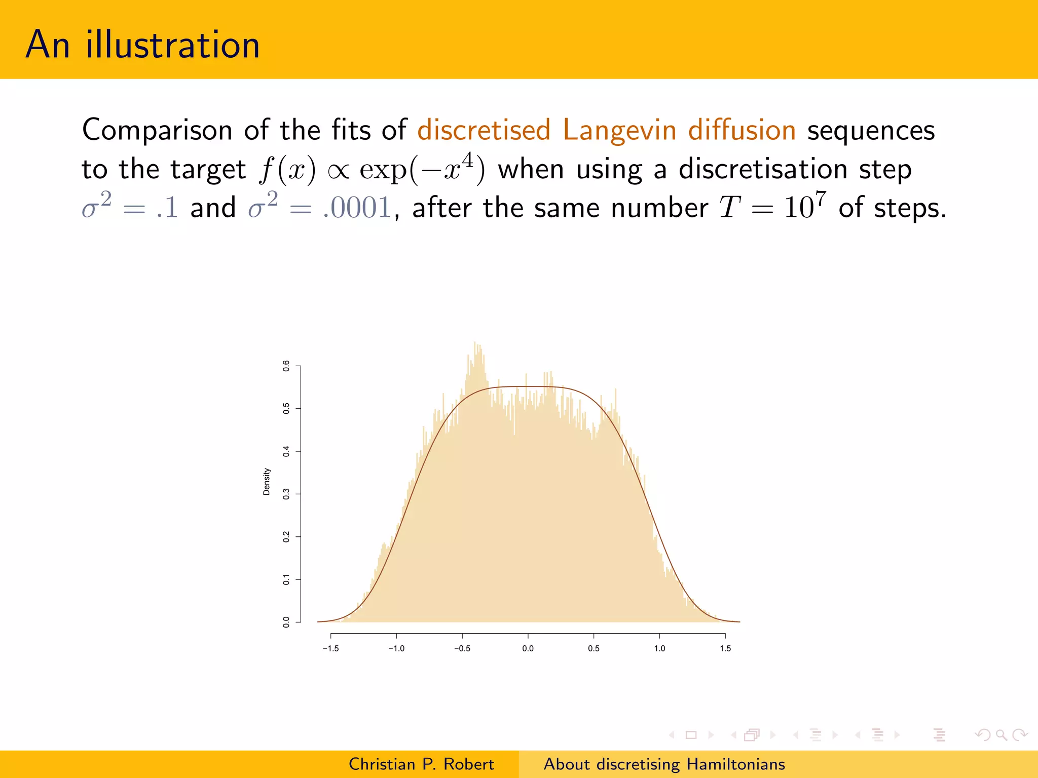
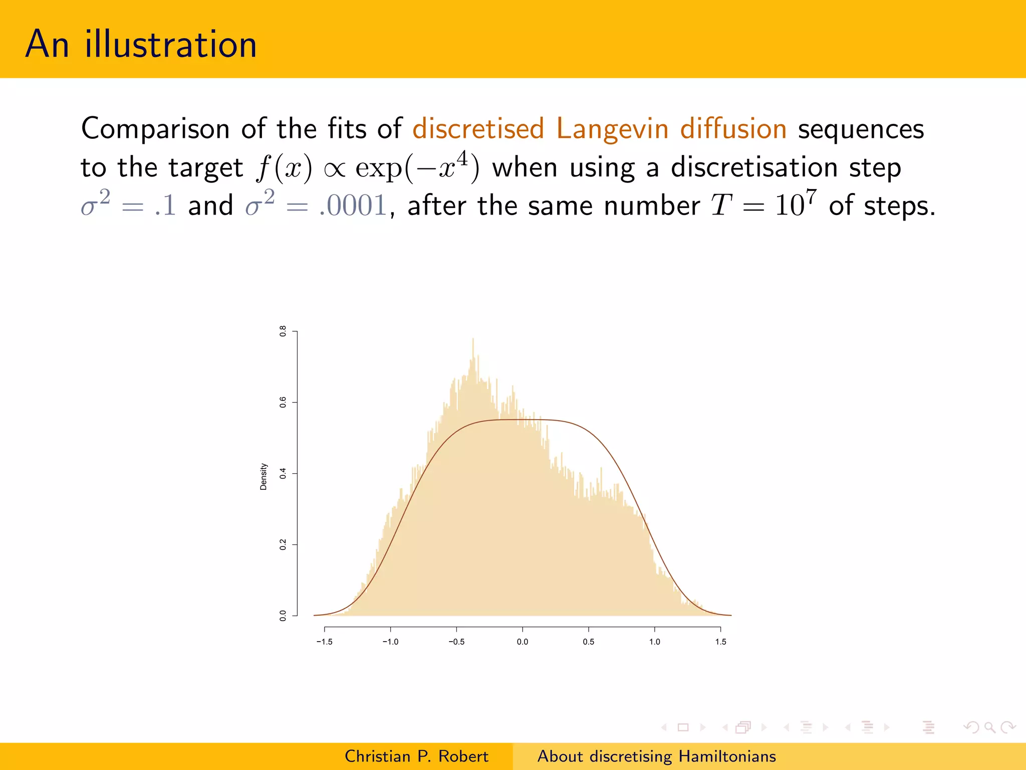
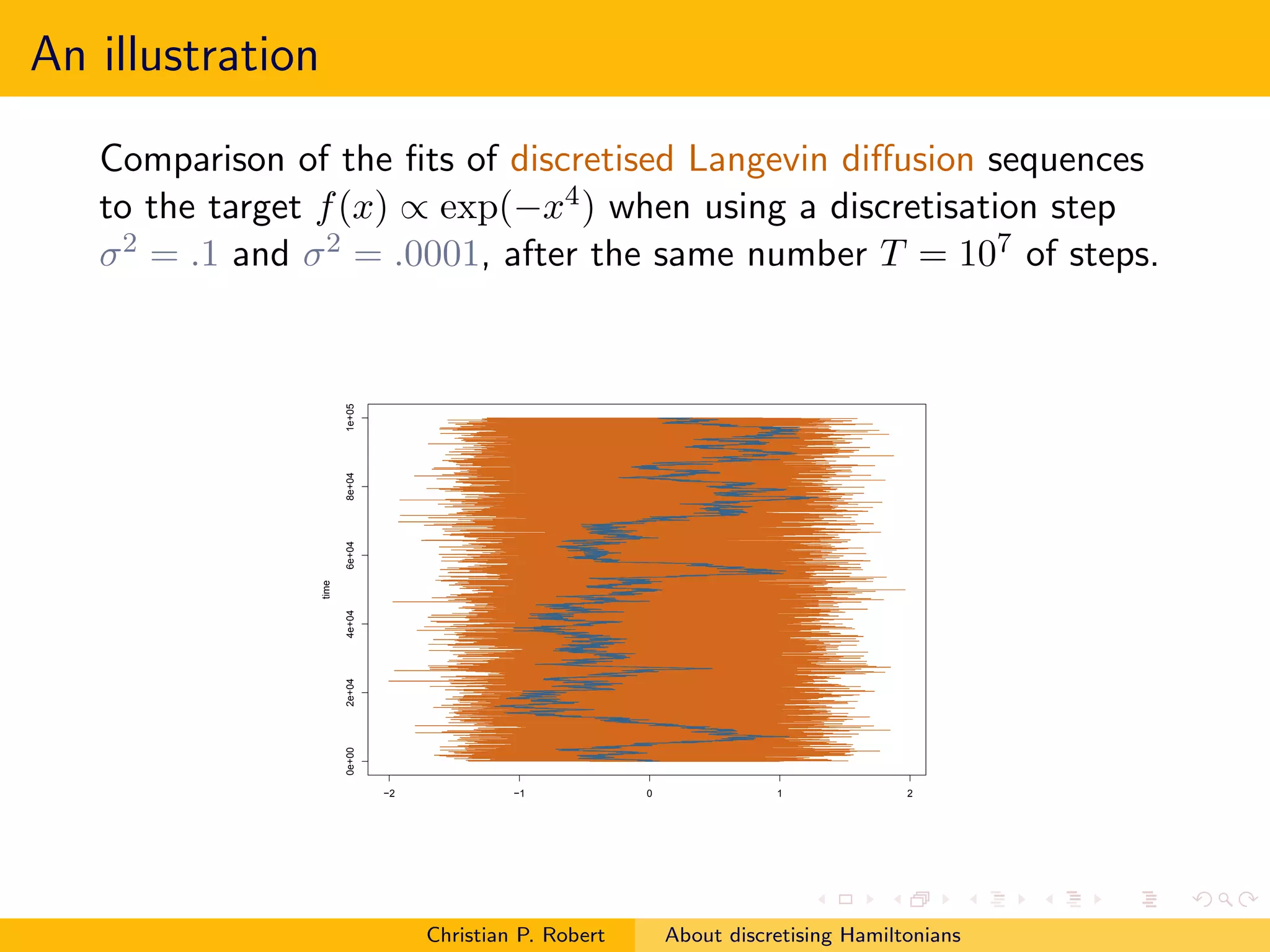
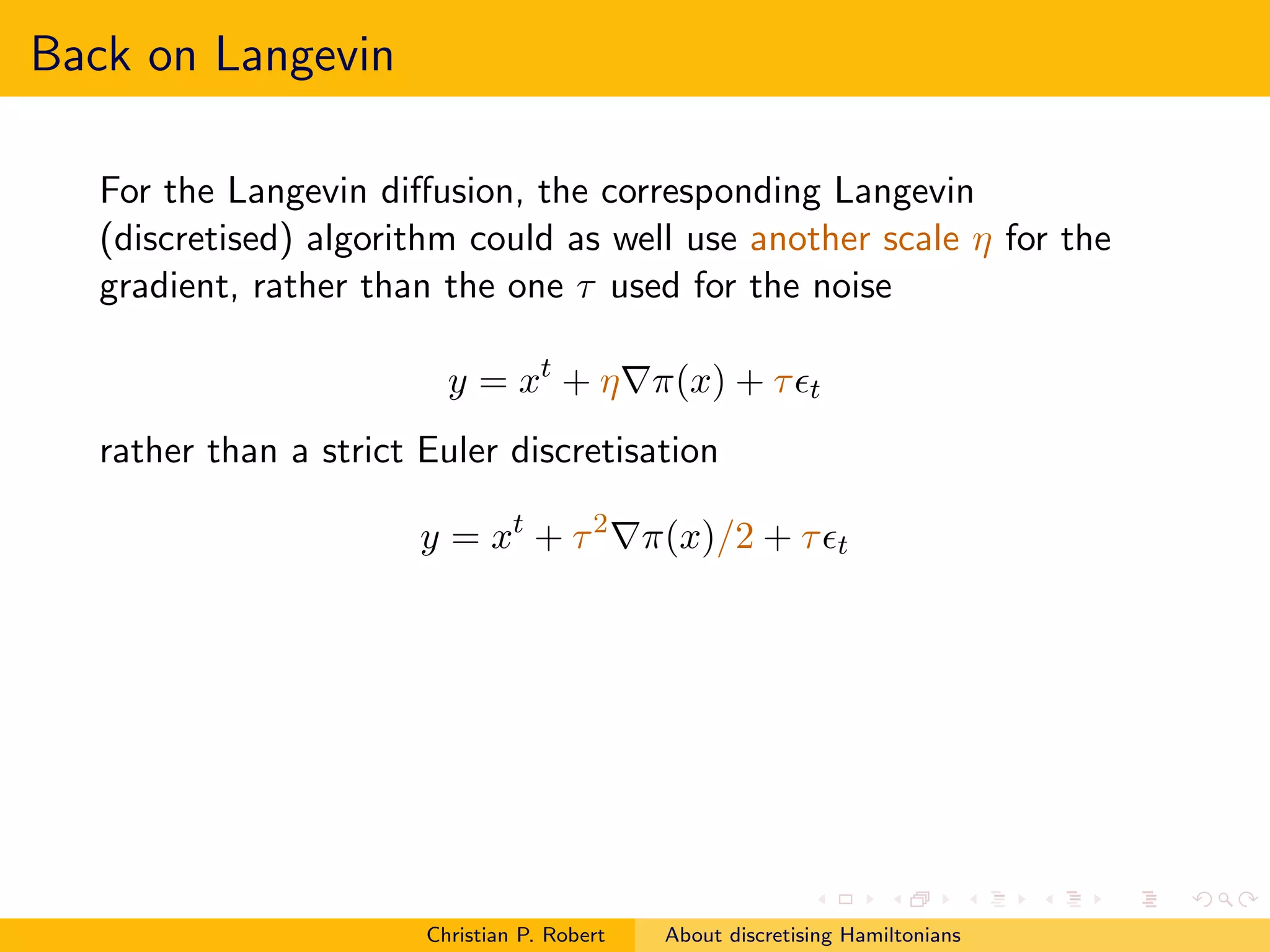
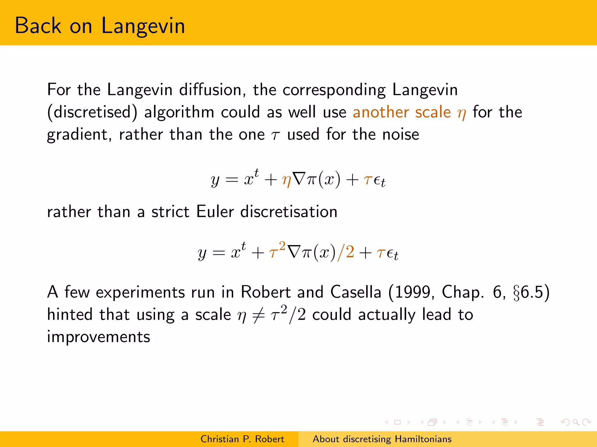
![Back on Langevin
For the Langevin diffusion, the corresponding Langevin
(discretised) algorithm could as well use another scale η for the
gradient, rather than the one τ used for the noise
y = xt + η∇π(x) + τ ǫt
rather than a strict Euler discretisation
y = xt + τ 2 ∇π(x)/2 + τ ǫt
A few experiments run in Robert and Casella (1999, Chap. 6, §6.5)
hinted that using a scale η = τ 2 /2 could actually lead to
improvements
Which [independent] framework should we adopt for
assessing discretised diffusions?
Christian P. Robert About discretising Hamiltonians](https://image.slidesharecdn.com/rs1013-coms-101013153858-phpapp02/75/RSS-discussion-of-Girolami-and-Calderhead-October-13-2010-13-2048.jpg)

1. The document discusses discretizing Hamiltonians for Markov chain Monte Carlo (MCMC) methods. Specifically, it examines reproducing Hamiltonian equations through discretization, such as via generalized leapfrog. 2. However, the invariance and stability properties of the continuous-time process may not carry over to the discretized version. Approximations can be corrected with a Metropolis-Hastings step, so exactly reproducing the continuous behavior is not necessarily useful. 3. Discretization induces a calibration problem of determining the appropriate step size. Convergence issues for the MCMC algorithm should not be impacted by imperfect renderings of the continuous-time process in discrete time.


