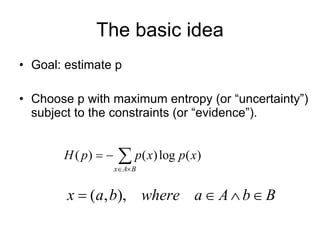
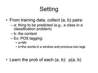
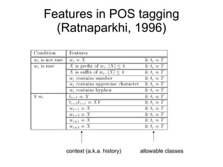
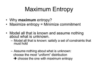
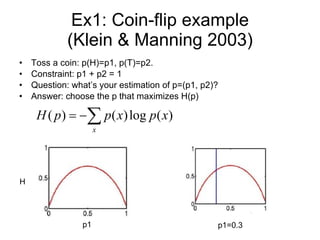
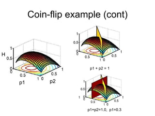
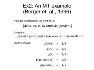
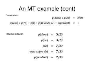
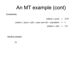
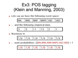
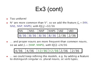
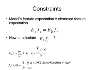
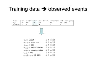
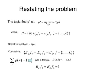
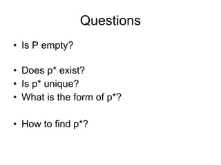
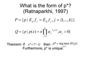
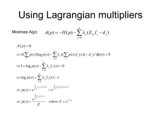
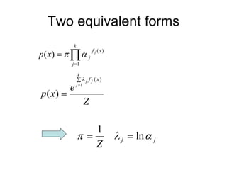
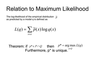
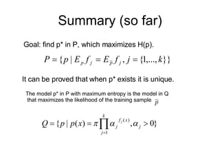
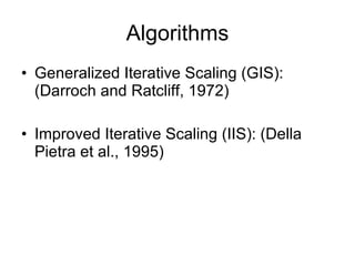
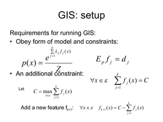
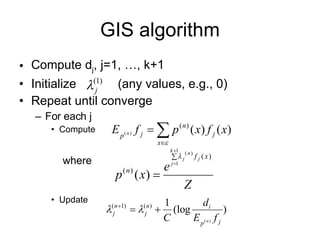
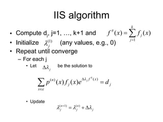
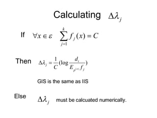
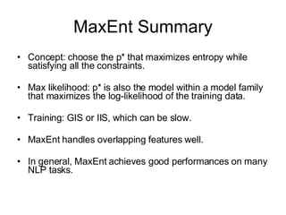
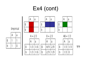
Maximum Entropy Model LING 572 Fei Xia 02/07-02/09/06
History The concept of Maximum Entropy can be traced back along multiple threads to Biblical times. Introduced  to NLP area  by Berger et. Al. (1996). Used in many NLP tasks: MT, Tagging, Parsing, PP attachment, LM, …
Outline Modeling: Intuition, basic concepts, … Parameter training Feature selection Case study
Reference papers (Ratnaparkhi, 1997) (Ratnaparkhi, 1996) (Berger et. al., 1996) (Klein and Manning, 2003)    Different notations.
Modeling
The basic idea Goal: estimate p Choose p with maximum entropy (or “uncertainty”) subject to the constraints (or “evidence”).
Setting From training data, collect (a, b) pairs: a: thing to be predicted (e.g., a class in a classification problem) b: the context Ex: POS tagging:  a=NN b=the words in a window and previous two tags Learn the prob of each (a, b):  p(a, b)
Features in POS tagging (Ratnaparkhi, 1996) context (a.k.a. history) allowable classes
Maximum Entropy Why  maximum  entropy? Maximize entropy = Minimize commitment Model all that is known and assume nothing about what is unknown.  Model all that is known: satisfy a set of constraints that must hold Assume nothing about what is unknown:  choose the most “uniform” distribution     choose the one with maximum entropy
Ex1: Coin-flip example (Klein & Manning 2003) Toss a coin: p(H)=p1, p(T)=p2. Constraint: p1 + p2 = 1 Question: what’s your estimation of p=(p1, p2)? Answer: choose the p that maximizes H(p) p1 H p1=0.3
Coin-flip example (cont) p1 p2 H p1 + p2 = 1 p1+p2=1.0,  p1=0.3
Ex2: An MT example (Berger et. al., 1996) Possible translation for the word “in” is:  Constraint: Intuitive answer:
An MT example (cont) Constraints: Intuitive answer:
An MT example (cont) Constraints: Intuitive answer:  ??
Ex3: POS tagging (Klein and Manning, 2003)
Ex3 (cont)
Ex4: overlapping features (Klein and Manning, 2003)
Modeling the problem Objective function: H(p) Goal: Among all the distributions that satisfy the constraints, choose the one, p*, that maximizes H(p). Question: How to represent constraints?
Features Feature (a.k.a. feature function, Indicator function) is a binary-valued function on events:  A: the set of possible classes (e.g., tags in POS tagging) B: space of contexts (e.g., neighboring words/ tags in POS tagging) Ex:
Some notations Finite training sample of events: Observed probability of x in S: The model p’s probability of x: Model expectation of  : Observed expectation of  : The j th  feature: (empirical count of  )
Constraints Model’s feature expectation = observed feature expectation How to calculate  ?
Training data    observed events
Restating the problem The task: find p* s.t.   where Objective function:  -H(p) Constraints:  Add a feature
Questions Is P empty? Does p* exist? Is p* unique? What is the form of p*?  How to find p*?
What is the form of p*? (Ratnaparkhi, 1997) Theorem: if  then  Furthermore, p* is unique.
Using Lagrangian multipliers Minimize A(p):
Two equivalent forms
Relation to Maximum Likelihood The log-likelihood of the empirical distribution  as predicted by a model q is defined as Theorem: if  then  Furthermore, p* is unique.
Summary (so far) The model p* in P with maximum entropy is the model in Q that maximizes the likelihood of the training sample  Goal: find p* in P, which maximizes H(p). It can be proved that when p* exists it is unique.
Summary (cont) Adding constraints (features): (Klein and Manning, 2003) Lower maximum entropy Raise maximum likelihood of data Bring the distribution further from uniform Bring the distribution closer to data
Parameter estimation
Algorithms Generalized Iterative Scaling (GIS): (Darroch and Ratcliff, 1972) Improved Iterative Scaling (IIS): (Della Pietra et al., 1995)
GIS: setup Requirements for running GIS: Obey form of model and constraints: An additional constraint: Let Add a new feature f k+1 :
GIS algorithm Compute d j , j=1, …, k+1 Initialize  (any values, e.g., 0)  Repeat until converge For each j Compute  Update where
Approximation for calculating feature expectation
Properties of GIS L(p (n+1) ) >= L(p (n) ) The sequence is guaranteed to converge to p*. The converge can be very slow. The running time of each iteration is O(NPA): N: the training set size P: the number of classes A: the average number of features that are active for a given event (a, b).
IIS algorithm Compute d j , j=1, …, k+1 and Initialize  (any values, e.g., 0)  Repeat until converge For each j Let  be the solution to  Update
Calculating  If Then GIS is the same as IIS Else must be calcuated numerically.
Feature selection
Feature selection Throw in many features and let the machine select the weights Manually specify feature templates Problem: too many features An alternative: greedy algorithm Start with an empty set S Add a feature at each iteration
Notation The gain in the log-likelihood of the training data: After adding a feature: With the feature set S:
Feature selection algorithm (Berger et al., 1996) Start with S being empty; thus p s  is uniform. Repeat until the gain is small enough For each candidate feature f Computer the model  using IIS Calculate the log-likelihood gain Choose the feature with maximal gain, and add it to S    Problem: too expensive
Approximating gains (Berger et. al., 1996)  Instead of recalculating all the weights, calculate only the weight of the new feature.
Training a MaxEnt Model Scenario #1: Define features templates Create the feature set Determine the optimum feature weights via GIS or IIS Scenario #2: Define feature templates Create candidate feature set S At every iteration, choose the feature from S (with max gain) and determine its weight (or choose top-n features and their weights).
Case study
POS tagging (Ratnaparkhi, 1996) Notation variation:  f j (a, b): a: class, b: context  f j (h i , t i ):  h: history for i th  word, t: tag for i th  word History: Training data: Treat it as a list of  (h i , t i ) pairs. How many pairs are there?
Using a MaxEnt Model Modeling:  Training:  Define features templates Create the feature set Determine the optimum feature weights via GIS or IIS Decoding:
Modeling
Training step 1:  define feature templates History h i Tag t i
Step 2: Create feature set Collect all the features from the training data Throw away features that appear less than 10 times
Step 3: determine the feature weights GIS Training time: Each iteration: O(NTA): N: the training set size T: the number of allowable tags A: average number of features that are active for a (h, t). About 24 hours on an IBM RS/6000 Model 380. How many features?
Decoding: Beam search Generate tags for w 1 , find top N, set s 1j  accordingly, j=1, 2, …, N For i=2 to n (n is the sentence length) For j=1 to N Generate tags for wi, given s (i-1)j  as previous tag context Append each tag to s (i-1)j  to make a new sequence. Find N highest prob sequences generated above, and set s ij  accordingly, j=1, …, N Return highest prob sequence s n1 .
Beam search
Viterbi search
Decoding (cont) Tags for words: Known words: use tag dictionary Unknown words: try all possible tags Ex: “time flies like an arrow” Running time: O(NTAB) N: sentence length B: beam size T: tagset size A: average number of features that are active for a given event
Experiment results
Comparison with other learners HMM: MaxEnt uses more context SDT:  MaxEnt does not split data TBL:  MaxEnt is statistical and it provides probability distributions.
MaxEnt Summary Concept: choose the p* that maximizes entropy while satisfying all the constraints. Max likelihood: p* is also the model within a model family that maximizes the log-likelihood of the training data. Training: GIS or IIS, which can be slow. MaxEnt handles overlapping features well. In general, MaxEnt achieves good performances on many NLP tasks.
Additional slides
Ex4 (cont) ??

Max Entropy

  • 1.
    Maximum Entropy ModelLING 572 Fei Xia 02/07-02/09/06
  • 2.
    History The conceptof Maximum Entropy can be traced back along multiple threads to Biblical times. Introduced to NLP area by Berger et. Al. (1996). Used in many NLP tasks: MT, Tagging, Parsing, PP attachment, LM, …
  • 3.
    Outline Modeling: Intuition,basic concepts, … Parameter training Feature selection Case study
  • 4.
    Reference papers (Ratnaparkhi,1997) (Ratnaparkhi, 1996) (Berger et. al., 1996) (Klein and Manning, 2003)  Different notations.
  • 5.
  • 6.
    The basic ideaGoal: estimate p Choose p with maximum entropy (or “uncertainty”) subject to the constraints (or “evidence”).
  • 7.
    Setting From trainingdata, collect (a, b) pairs: a: thing to be predicted (e.g., a class in a classification problem) b: the context Ex: POS tagging: a=NN b=the words in a window and previous two tags Learn the prob of each (a, b): p(a, b)
  • 8.
    Features in POStagging (Ratnaparkhi, 1996) context (a.k.a. history) allowable classes
  • 9.
    Maximum Entropy Why maximum entropy? Maximize entropy = Minimize commitment Model all that is known and assume nothing about what is unknown. Model all that is known: satisfy a set of constraints that must hold Assume nothing about what is unknown: choose the most “uniform” distribution  choose the one with maximum entropy
  • 10.
    Ex1: Coin-flip example(Klein & Manning 2003) Toss a coin: p(H)=p1, p(T)=p2. Constraint: p1 + p2 = 1 Question: what’s your estimation of p=(p1, p2)? Answer: choose the p that maximizes H(p) p1 H p1=0.3
  • 11.
    Coin-flip example (cont)p1 p2 H p1 + p2 = 1 p1+p2=1.0, p1=0.3
  • 12.
    Ex2: An MTexample (Berger et. al., 1996) Possible translation for the word “in” is: Constraint: Intuitive answer:
  • 13.
    An MT example(cont) Constraints: Intuitive answer:
  • 14.
    An MT example(cont) Constraints: Intuitive answer: ??
  • 15.
    Ex3: POS tagging(Klein and Manning, 2003)
  • 16.
  • 17.
    Ex4: overlapping features(Klein and Manning, 2003)
  • 18.
    Modeling the problemObjective function: H(p) Goal: Among all the distributions that satisfy the constraints, choose the one, p*, that maximizes H(p). Question: How to represent constraints?
  • 19.
    Features Feature (a.k.a.feature function, Indicator function) is a binary-valued function on events: A: the set of possible classes (e.g., tags in POS tagging) B: space of contexts (e.g., neighboring words/ tags in POS tagging) Ex:
  • 20.
    Some notations Finitetraining sample of events: Observed probability of x in S: The model p’s probability of x: Model expectation of : Observed expectation of : The j th feature: (empirical count of )
  • 21.
    Constraints Model’s featureexpectation = observed feature expectation How to calculate ?
  • 22.
    Training data  observed events
  • 23.
    Restating the problemThe task: find p* s.t. where Objective function: -H(p) Constraints: Add a feature
  • 24.
    Questions Is Pempty? Does p* exist? Is p* unique? What is the form of p*? How to find p*?
  • 25.
    What is theform of p*? (Ratnaparkhi, 1997) Theorem: if then Furthermore, p* is unique.
  • 26.
  • 27.
  • 28.
    Relation to MaximumLikelihood The log-likelihood of the empirical distribution as predicted by a model q is defined as Theorem: if then Furthermore, p* is unique.
  • 29.
    Summary (so far)The model p* in P with maximum entropy is the model in Q that maximizes the likelihood of the training sample Goal: find p* in P, which maximizes H(p). It can be proved that when p* exists it is unique.
  • 30.
    Summary (cont) Addingconstraints (features): (Klein and Manning, 2003) Lower maximum entropy Raise maximum likelihood of data Bring the distribution further from uniform Bring the distribution closer to data
  • 31.
  • 32.
    Algorithms Generalized IterativeScaling (GIS): (Darroch and Ratcliff, 1972) Improved Iterative Scaling (IIS): (Della Pietra et al., 1995)
  • 33.
    GIS: setup Requirementsfor running GIS: Obey form of model and constraints: An additional constraint: Let Add a new feature f k+1 :
  • 34.
    GIS algorithm Computed j , j=1, …, k+1 Initialize (any values, e.g., 0) Repeat until converge For each j Compute Update where
  • 35.
    Approximation for calculatingfeature expectation
  • 36.
    Properties of GISL(p (n+1) ) >= L(p (n) ) The sequence is guaranteed to converge to p*. The converge can be very slow. The running time of each iteration is O(NPA): N: the training set size P: the number of classes A: the average number of features that are active for a given event (a, b).
  • 37.
    IIS algorithm Computed j , j=1, …, k+1 and Initialize (any values, e.g., 0) Repeat until converge For each j Let be the solution to Update
  • 38.
    Calculating IfThen GIS is the same as IIS Else must be calcuated numerically.
  • 39.
  • 40.
    Feature selection Throwin many features and let the machine select the weights Manually specify feature templates Problem: too many features An alternative: greedy algorithm Start with an empty set S Add a feature at each iteration
  • 41.
    Notation The gainin the log-likelihood of the training data: After adding a feature: With the feature set S:
  • 42.
    Feature selection algorithm(Berger et al., 1996) Start with S being empty; thus p s is uniform. Repeat until the gain is small enough For each candidate feature f Computer the model using IIS Calculate the log-likelihood gain Choose the feature with maximal gain, and add it to S  Problem: too expensive
  • 43.
    Approximating gains (Bergeret. al., 1996) Instead of recalculating all the weights, calculate only the weight of the new feature.
  • 44.
    Training a MaxEntModel Scenario #1: Define features templates Create the feature set Determine the optimum feature weights via GIS or IIS Scenario #2: Define feature templates Create candidate feature set S At every iteration, choose the feature from S (with max gain) and determine its weight (or choose top-n features and their weights).
  • 45.
  • 46.
    POS tagging (Ratnaparkhi,1996) Notation variation: f j (a, b): a: class, b: context f j (h i , t i ): h: history for i th word, t: tag for i th word History: Training data: Treat it as a list of (h i , t i ) pairs. How many pairs are there?
  • 47.
    Using a MaxEntModel Modeling: Training: Define features templates Create the feature set Determine the optimum feature weights via GIS or IIS Decoding:
  • 48.
  • 49.
    Training step 1: define feature templates History h i Tag t i
  • 50.
    Step 2: Createfeature set Collect all the features from the training data Throw away features that appear less than 10 times
  • 51.
    Step 3: determinethe feature weights GIS Training time: Each iteration: O(NTA): N: the training set size T: the number of allowable tags A: average number of features that are active for a (h, t). About 24 hours on an IBM RS/6000 Model 380. How many features?
  • 52.
    Decoding: Beam searchGenerate tags for w 1 , find top N, set s 1j accordingly, j=1, 2, …, N For i=2 to n (n is the sentence length) For j=1 to N Generate tags for wi, given s (i-1)j as previous tag context Append each tag to s (i-1)j to make a new sequence. Find N highest prob sequences generated above, and set s ij accordingly, j=1, …, N Return highest prob sequence s n1 .
  • 53.
  • 54.
  • 55.
    Decoding (cont) Tagsfor words: Known words: use tag dictionary Unknown words: try all possible tags Ex: “time flies like an arrow” Running time: O(NTAB) N: sentence length B: beam size T: tagset size A: average number of features that are active for a given event
  • 56.
  • 57.
    Comparison with otherlearners HMM: MaxEnt uses more context SDT: MaxEnt does not split data TBL: MaxEnt is statistical and it provides probability distributions.
  • 58.
    MaxEnt Summary Concept:choose the p* that maximizes entropy while satisfying all the constraints. Max likelihood: p* is also the model within a model family that maximizes the log-likelihood of the training data. Training: GIS or IIS, which can be slow. MaxEnt handles overlapping features well. In general, MaxEnt achieves good performances on many NLP tasks.
  • 59.
  • 60.