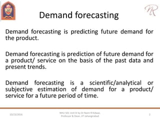
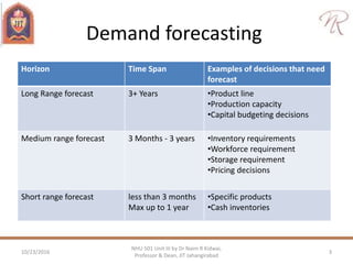
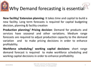
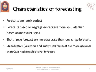
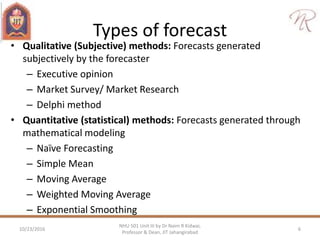
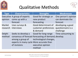
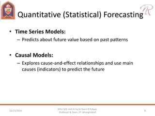
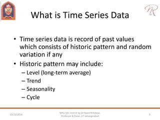
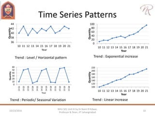
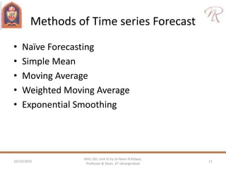
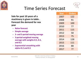
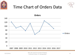
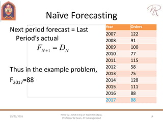
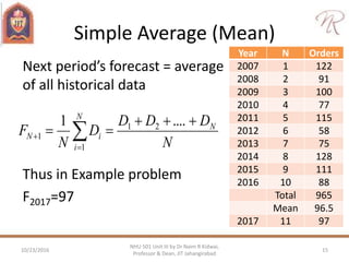
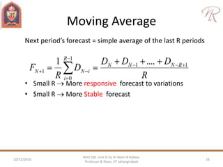
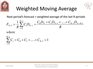
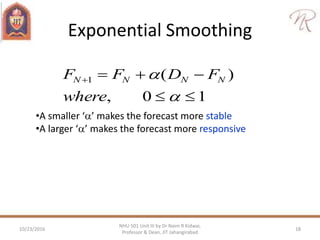
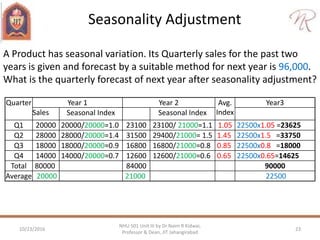
Demand Forecasting and Cost
Estimation
Characteristics of Forecasts, Forecasting Horizons, Steps to Forecasting,
Forecasting Methods, Seasonal Adjustments, Forecasting Performance Measures
Cost Estimation, Elements of cost, Computation of Material Variances Break‐Even Analysi
s
10/23/2016 1
NHU 501 Unit III by Dr Naim R Kidwai,
Professor & Dean, JIT Jahangirabad
Demand forecasting
Demand forecasting is predicting future demand for
the product.
Demand forecasting is prediction of future demand for
a product/ service on the basis of the past data and
present trends.
Demand forecasting is a scientific/analytical or
subjective estimation of demand for a product/
service for a future period of time.
10/23/2016 2
NHU 501 Unit III by Dr Naim R Kidwai,
Professor & Dean, JIT Jahangirabad
Demand forecasting
10/23/2016 3
NHU 501 Unit III by Dr Naim R Kidwai,
Professor & Dean, JIT Jahangirabad
Horizon Time Span Examples of decisions that need
forecast
Long Range forecast 3+ Years •Product line
•Production capacity
•Capital budgeting decisions
Medium range forecast 3 Months - 3 years •Inventory requirements
•Workforce requirement
•Storage requirement
•Pricing decisions
Short range forecast less than 3 months
Max up to 1 year
•Specific products
•Cash inventories
Why Demand forecasting is essential
New facility/ Extension planning: It takes time and capital to build a
new facility. Long term forecasts is required for capital budgeting
decision, planning & facility creation
Production planning/ Pricing decision: Demand for products and
services have seasonal and other variations. Medium range
forecasts are required to adjust production capacity to the demand
variation and to make pricing decisions in order to enhance
profitability.
Workforce scheduling/ working capital decisions: short range
demand forecast is required to make workforce scheduling and
working capital decisions in order to enhance profitability
10/23/2016 4
NHU 501 Unit III by Dr Naim R Kidwai,
Professor & Dean, JIT Jahangirabad
Characteristics of forecasting
• Forecasts are rarely perfect
• Forecasts based on aggregated data are more accurate than
based on individual items
• Short range forecast are more accurate than long range forecasts
• Quantitative (Scientific and analytical) forecast are more accurate
than Qualitative (subjective) forecast
10/23/2016 5
NHU 501 Unit III by Dr Naim R Kidwai,
Professor & Dean, JIT Jahangirabad
Types of forecast
• Qualitative (Subjective) methods: Forecasts generated
subjectively by the forecaster
– Executive opinion
– Market Survey/ Market Research
– Delphi method
• Quantitative (statistical) methods: Forecasts generated through
mathematical modeling
– Naïve Forecasting
– Simple Mean
– Moving Average
– Weighted Moving Average
– Exponential Smoothing
10/23/2016 6
NHU 501 Unit III by Dr Naim R Kidwai,
Professor & Dean, JIT Jahangirabad
Qualitative Methods
Type Characteristics Strengths Weaknesses
Executive
opinion
A group of experts
come up with a
forecast
Good for strategic or
new-product
forecasting
One person's opinion
can dominate the
forecast
Market
research
Uses surveys &
interviews
Good determinant of
customer preferences
& demand
developing a good
questionnaire is a
challenge
Delphi
method
Seeks to develop a
consensus of forecast
among a group of
experts in many cycle
of revisions
Good for long-range
forecasting of demand,
technological changes,
More accurate than
executive opinion
method
Time consuming to
develop.
10/23/2016 7
NHU 501 Unit III by Dr Naim R Kidwai,
Professor & Dean, JIT Jahangirabad
Quantitative (Statistical) Forecasting
• Time Series Models:
– Predicts about future value based on past patterns
• Causal Models:
– Explores cause-and-effect relationships and use main
causes (indicators) to predict the future
10/23/2016 8
NHU 501 Unit III by Dr Naim R Kidwai,
Professor & Dean, JIT Jahangirabad
What is Time Series Data
• Time series data is record of past values
which consists of historic pattern and random
variation if any
• Historic pattern may include:
– Level (long-term average)
– Trend
– Seasonality
– Cycle
10/23/2016 9
NHU 501 Unit III by Dr Naim R Kidwai,
Professor & Dean, JIT Jahangirabad
Time Series Patterns
36
38
40
42
44
10 11 12 13 14 15 16 17 18 19 20 21
Quantity
Year
0
20
40
60
80
100
10 11 12 13 14 15 16 17 18 19 20 21
Quantity
Year
0
10
20
30
40
50
60
13Q1
13Q2
13Q3
13Q4
14Q1
14Q2
14Q3
14Q4
15Q1
15Q2
15Q3
15Q4
Quantity
Year
100
120
140
160
180
200
220
10 11 12 13 14 15 16 17 18 19 20 21
Quantity
Year
Trend : Exponential increaseTrend : Level / Horizontal pattern
Trend : Linear increaseTrend : Periodic/ Seasonal Variation
10/23/2016 10
NHU 501 Unit III by Dr Naim R Kidwai,
Professor & Dean, JIT Jahangirabad
Methods of Time series Forecast
• Naïve Forecasting
• Simple Mean
• Moving Average
• Weighted Moving Average
• Exponential Smoothing
10/23/2016 11
NHU 501 Unit III by Dr Naim R Kidwai,
Professor & Dean, JIT Jahangirabad
Time Series Forecast
Sale for past 10 years of a
machinery is given in table .
Forecast the demand for nex
year
– Naïve forecast
– Simple average
– 3- and 5-period moving average
– 3-period weighted moving
average with weights 0.5, 0.3,
and 0.2
– Exponential smoothing with
alpha=0.2 and 0.5
Year Orders
2007 122
2008 91
2009 100
2010 77
2011 115
2012 58
2013 75
2014 128
2015 111
2016 88
2017 ??
10/23/2016 12
NHU 501 Unit III by Dr Naim R Kidwai,
Professor & Dean, JIT Jahangirabad
Time Chart of Orders Data
0
20
40
60
80
100
120
140
2007 2008 2009 2010 2011 2012 2013 2014 2015 2016 2017
Orders
Orders
10/23/2016 13
NHU 501 Unit III by Dr Naim R Kidwai,
Professor & Dean, JIT Jahangirabad
Naïve Forecasting
Next period forecast = Last
Period’s actual
Thus in the example problem,
F2017=88
NN DF 1
Year Orders
2007 122
2008 91
2009 100
2010 77
2011 115
2012 58
2013 75
2014 128
2015 111
2016 88
2017 88
10/23/2016 14
NHU 501 Unit III by Dr Naim R Kidwai,
Professor & Dean, JIT Jahangirabad
Simple Average (Mean)
Next period’s forecast = average
of all historical data
Thus in Example problem
F2017=97
N
DDD
D
N
F N
N
i
iN

 

....1 21
1
1
Year N Orders
2007 1 122
2008 2 91
2009 3 100
2010 4 77
2011 5 115
2012 6 58
2013 7 75
2014 8 128
2015 9 111
2016 10 88
Total 965
Mean 96.5
2017 11 97
10/23/2016 15
NHU 501 Unit III by Dr Naim R Kidwai,
Professor & Dean, JIT Jahangirabad
Moving Average
Next period’s forecast = simple average of the last R periods
• Small R  More responsive forecast to variations
• Small R  More Stable forecast
R
DDD
D
R
F RNNN
R
i
iNN
11
1
0
1
....1 




 
10/23/2016 16
NHU 501 Unit III by Dr Naim R Kidwai,
Professor & Dean, JIT Jahangirabad
Weighted Moving Average
Next period’s forecast = weighted average of the last R periods
1....
....1
110
1
0
11110
1
0
1












R
R
i
i
RNRNN
R
i
iNiN
CCCC
where
R
DCDCDC
DC
R
F
10/23/2016 17
NHU 501 Unit III by Dr Naim R Kidwai,
Professor & Dean, JIT Jahangirabad
Exponential Smoothing
10,
)(1




where
FDFF NNNN
•A smaller ‘’ makes the forecast more stable
•A larger ‘’ makes the forecast more responsive
10/23/2016 18
NHU 501 Unit III by Dr Naim R Kidwai,
Professor & Dean, JIT Jahangirabad
Exponential Smoothing
Period
Orders
Naïveforecast
SimpleAverage
MovingAverage
(N=3)
MovingAverage
(N=5)
WeightedMoving
Average(N=3)
Weights:0.5,0.3,
0.2
WeightedMoving
Average(N=3)
Weights:0.6,0.3,
0.1
Exponential
Smoothening
(alpha=0.2)
Exponential
Smoothening
(alpha=0.5)
2007 122 122 122
2008 91 122 122 122 122
2009 100 91 107 116 107
2010 77 100 104 104 102 100 113 104
2011 115 77 98 89 87 85 106 91
2012 58 115 101 97 101 101 102 108 103
2013 75 58 94 83 88 79 77 98 81
2014 128 75 91 83 85 78 74 93 78
2015 111 128 96 87 91 98 105 100 103
2016 88 111 97 105 97 109 113 102 107
88 97 109 92 103 99 99 98
10/23/2016 19
NHU 501 Unit III by Dr Naim R Kidwai,
Professor & Dean, JIT Jahangirabad
Forecast Accuracy measures
• Forecasts are rarely perfect so we need to know how
much we should rely on our chosen forecasting method
• Measuring forecast error: EN=DN-FN
• Note that over forecasts  negative errors
and under forecasts  positive errors
• Mean Absolute Deviation (MAD):
– A good measure of the actual error in a forecast
• Mean Square Error (MSE):
– Penalizes extreme errors
Method for which any of measures of error is least
10/23/2016 20
NHU 501 Unit III by Dr Naim R Kidwai,
Professor & Dean, JIT Jahangirabad


N
i
ii FD
N
MAD
1
1
 

N
i
ii FD
N
MSE
1
21
Exponential Smoothing
Period
Orders
Naïveforecast
Simple
Average
Moving
Average(N=3)
Moving
Average(N=5)
Weighted
Moving
Average(N=3)
Weights:0.5,
0.3,0.2
Weighted
Moving
Average(N=3)
Weights:0.6,
0.3,0.1
Exponential
Smoothening
(alpha=0.2)
Exponential
Smoothening
(alpha=0.5)
2007 122 122 122
2008 91 122 122 122 122
2009 100 91 107 116 107
2010 77 100 104 104 102 100 113 104
2011 115 77 98 89 87 85 106 91
2012 58 115 101 97 101 101 102 108 103
2013 75 58 94 83 88 79 77 98 81
2014 128 75 91 83 85 78 74 93 78
2015 111 128 96 87 91 98 105 100 103
2016 88 111 97 105 97 109 113 102 107
2017 Forecast 88 97 109 92 103 99 99 98
MAD 28 22 23 22 24 25 26 23
MSE 1131 657 840 870 912 992 796 811
10/23/2016 21
NHU 501 Unit III by Dr Naim R Kidwai,
Professor & Dean, JIT Jahangirabad
Seasonal Adjustment
Steps for seasonal adjustment in forecast
• Calculate the average demand per season
– E.g.: average quarterly demand
• Calculate a seasonal index for each season of each year:
– (Demand of season /Average demand per season of the year
• Average the indexes by season
– E.g.: take the average of all winter indexes, Summer indexes, ...
• Forecast demand for the next year & divide by the number of seasons
– Use regular forecasting method & divide by four for average quarterly demand
• Multiply next year’s average seasonal demand by each average
seasonal index
– Result is a forecast of demand for each season of next year
10/23/2016 22
NHU 501 Unit III by Dr Naim R Kidwai,
Professor & Dean, JIT Jahangirabad
A Product has seasonal variation. Its Quarterly sales for the past two
years is given and forecast by a suitable method for next year is 96,000.
What is the quarterly forecast of next year after seasonality adjustment?
10/23/2016 23
NHU 501 Unit III by Dr Naim R Kidwai,
Professor & Dean, JIT Jahangirabad
Seasonality Adjustment
Quarter Year 1 Year 2 Avg.
Index
Year3
Sales Seasonal Index Seasonal Index
Q1 20000 20000/20000=1.0 23100 23100/ 21000=1.1 1.05 22500x1.05 =23625
Q2 28000 28000/20000=1.4 31500 29400/21000= 1.5 1.45 22500x1.5 =33750
Q3 18000 18000/20000=0.9 16800 16800/21000=0.8 0.85 22500x0.8 =18000
Q4 14000 14000/20000=0.7 12600 12600/21000=0.6 0.65 22500x0.65=14625
Total 80000 84000 90000
Average 20000 21000 22500

demand forecasting

  • 1.
    Demand Forecasting andCost Estimation Characteristics of Forecasts, Forecasting Horizons, Steps to Forecasting, Forecasting Methods, Seasonal Adjustments, Forecasting Performance Measures Cost Estimation, Elements of cost, Computation of Material Variances Break‐Even Analysi s 10/23/2016 1 NHU 501 Unit III by Dr Naim R Kidwai, Professor & Dean, JIT Jahangirabad
  • 2.
    Demand forecasting Demand forecastingis predicting future demand for the product. Demand forecasting is prediction of future demand for a product/ service on the basis of the past data and present trends. Demand forecasting is a scientific/analytical or subjective estimation of demand for a product/ service for a future period of time. 10/23/2016 2 NHU 501 Unit III by Dr Naim R Kidwai, Professor & Dean, JIT Jahangirabad
  • 3.
    Demand forecasting 10/23/2016 3 NHU501 Unit III by Dr Naim R Kidwai, Professor & Dean, JIT Jahangirabad Horizon Time Span Examples of decisions that need forecast Long Range forecast 3+ Years •Product line •Production capacity •Capital budgeting decisions Medium range forecast 3 Months - 3 years •Inventory requirements •Workforce requirement •Storage requirement •Pricing decisions Short range forecast less than 3 months Max up to 1 year •Specific products •Cash inventories
  • 4.
    Why Demand forecastingis essential New facility/ Extension planning: It takes time and capital to build a new facility. Long term forecasts is required for capital budgeting decision, planning & facility creation Production planning/ Pricing decision: Demand for products and services have seasonal and other variations. Medium range forecasts are required to adjust production capacity to the demand variation and to make pricing decisions in order to enhance profitability. Workforce scheduling/ working capital decisions: short range demand forecast is required to make workforce scheduling and working capital decisions in order to enhance profitability 10/23/2016 4 NHU 501 Unit III by Dr Naim R Kidwai, Professor & Dean, JIT Jahangirabad
  • 5.
    Characteristics of forecasting •Forecasts are rarely perfect • Forecasts based on aggregated data are more accurate than based on individual items • Short range forecast are more accurate than long range forecasts • Quantitative (Scientific and analytical) forecast are more accurate than Qualitative (subjective) forecast 10/23/2016 5 NHU 501 Unit III by Dr Naim R Kidwai, Professor & Dean, JIT Jahangirabad
  • 6.
    Types of forecast •Qualitative (Subjective) methods: Forecasts generated subjectively by the forecaster – Executive opinion – Market Survey/ Market Research – Delphi method • Quantitative (statistical) methods: Forecasts generated through mathematical modeling – Naïve Forecasting – Simple Mean – Moving Average – Weighted Moving Average – Exponential Smoothing 10/23/2016 6 NHU 501 Unit III by Dr Naim R Kidwai, Professor & Dean, JIT Jahangirabad
  • 7.
    Qualitative Methods Type CharacteristicsStrengths Weaknesses Executive opinion A group of experts come up with a forecast Good for strategic or new-product forecasting One person's opinion can dominate the forecast Market research Uses surveys & interviews Good determinant of customer preferences & demand developing a good questionnaire is a challenge Delphi method Seeks to develop a consensus of forecast among a group of experts in many cycle of revisions Good for long-range forecasting of demand, technological changes, More accurate than executive opinion method Time consuming to develop. 10/23/2016 7 NHU 501 Unit III by Dr Naim R Kidwai, Professor & Dean, JIT Jahangirabad
  • 8.
    Quantitative (Statistical) Forecasting •Time Series Models: – Predicts about future value based on past patterns • Causal Models: – Explores cause-and-effect relationships and use main causes (indicators) to predict the future 10/23/2016 8 NHU 501 Unit III by Dr Naim R Kidwai, Professor & Dean, JIT Jahangirabad
  • 9.
    What is TimeSeries Data • Time series data is record of past values which consists of historic pattern and random variation if any • Historic pattern may include: – Level (long-term average) – Trend – Seasonality – Cycle 10/23/2016 9 NHU 501 Unit III by Dr Naim R Kidwai, Professor & Dean, JIT Jahangirabad
  • 10.
    Time Series Patterns 36 38 40 42 44 1011 12 13 14 15 16 17 18 19 20 21 Quantity Year 0 20 40 60 80 100 10 11 12 13 14 15 16 17 18 19 20 21 Quantity Year 0 10 20 30 40 50 60 13Q1 13Q2 13Q3 13Q4 14Q1 14Q2 14Q3 14Q4 15Q1 15Q2 15Q3 15Q4 Quantity Year 100 120 140 160 180 200 220 10 11 12 13 14 15 16 17 18 19 20 21 Quantity Year Trend : Exponential increaseTrend : Level / Horizontal pattern Trend : Linear increaseTrend : Periodic/ Seasonal Variation 10/23/2016 10 NHU 501 Unit III by Dr Naim R Kidwai, Professor & Dean, JIT Jahangirabad
  • 11.
    Methods of Timeseries Forecast • Naïve Forecasting • Simple Mean • Moving Average • Weighted Moving Average • Exponential Smoothing 10/23/2016 11 NHU 501 Unit III by Dr Naim R Kidwai, Professor & Dean, JIT Jahangirabad
  • 12.
    Time Series Forecast Salefor past 10 years of a machinery is given in table . Forecast the demand for nex year – Naïve forecast – Simple average – 3- and 5-period moving average – 3-period weighted moving average with weights 0.5, 0.3, and 0.2 – Exponential smoothing with alpha=0.2 and 0.5 Year Orders 2007 122 2008 91 2009 100 2010 77 2011 115 2012 58 2013 75 2014 128 2015 111 2016 88 2017 ?? 10/23/2016 12 NHU 501 Unit III by Dr Naim R Kidwai, Professor & Dean, JIT Jahangirabad
  • 13.
    Time Chart ofOrders Data 0 20 40 60 80 100 120 140 2007 2008 2009 2010 2011 2012 2013 2014 2015 2016 2017 Orders Orders 10/23/2016 13 NHU 501 Unit III by Dr Naim R Kidwai, Professor & Dean, JIT Jahangirabad
  • 14.
    Naïve Forecasting Next periodforecast = Last Period’s actual Thus in the example problem, F2017=88 NN DF 1 Year Orders 2007 122 2008 91 2009 100 2010 77 2011 115 2012 58 2013 75 2014 128 2015 111 2016 88 2017 88 10/23/2016 14 NHU 501 Unit III by Dr Naim R Kidwai, Professor & Dean, JIT Jahangirabad
  • 15.
    Simple Average (Mean) Nextperiod’s forecast = average of all historical data Thus in Example problem F2017=97 N DDD D N F N N i iN     ....1 21 1 1 Year N Orders 2007 1 122 2008 2 91 2009 3 100 2010 4 77 2011 5 115 2012 6 58 2013 7 75 2014 8 128 2015 9 111 2016 10 88 Total 965 Mean 96.5 2017 11 97 10/23/2016 15 NHU 501 Unit III by Dr Naim R Kidwai, Professor & Dean, JIT Jahangirabad
  • 16.
    Moving Average Next period’sforecast = simple average of the last R periods • Small R  More responsive forecast to variations • Small R  More Stable forecast R DDD D R F RNNN R i iNN 11 1 0 1 ....1        10/23/2016 16 NHU 501 Unit III by Dr Naim R Kidwai, Professor & Dean, JIT Jahangirabad
  • 17.
    Weighted Moving Average Nextperiod’s forecast = weighted average of the last R periods 1.... ....1 110 1 0 11110 1 0 1             R R i i RNRNN R i iNiN CCCC where R DCDCDC DC R F 10/23/2016 17 NHU 501 Unit III by Dr Naim R Kidwai, Professor & Dean, JIT Jahangirabad
  • 18.
    Exponential Smoothing 10, )(1     where FDFF NNNN •Asmaller ‘’ makes the forecast more stable •A larger ‘’ makes the forecast more responsive 10/23/2016 18 NHU 501 Unit III by Dr Naim R Kidwai, Professor & Dean, JIT Jahangirabad
  • 19.
    Exponential Smoothing Period Orders Naïveforecast SimpleAverage MovingAverage (N=3) MovingAverage (N=5) WeightedMoving Average(N=3) Weights:0.5,0.3, 0.2 WeightedMoving Average(N=3) Weights:0.6,0.3, 0.1 Exponential Smoothening (alpha=0.2) Exponential Smoothening (alpha=0.5) 2007 122122 122 2008 91 122 122 122 122 2009 100 91 107 116 107 2010 77 100 104 104 102 100 113 104 2011 115 77 98 89 87 85 106 91 2012 58 115 101 97 101 101 102 108 103 2013 75 58 94 83 88 79 77 98 81 2014 128 75 91 83 85 78 74 93 78 2015 111 128 96 87 91 98 105 100 103 2016 88 111 97 105 97 109 113 102 107 88 97 109 92 103 99 99 98 10/23/2016 19 NHU 501 Unit III by Dr Naim R Kidwai, Professor & Dean, JIT Jahangirabad
  • 20.
    Forecast Accuracy measures •Forecasts are rarely perfect so we need to know how much we should rely on our chosen forecasting method • Measuring forecast error: EN=DN-FN • Note that over forecasts  negative errors and under forecasts  positive errors • Mean Absolute Deviation (MAD): – A good measure of the actual error in a forecast • Mean Square Error (MSE): – Penalizes extreme errors Method for which any of measures of error is least 10/23/2016 20 NHU 501 Unit III by Dr Naim R Kidwai, Professor & Dean, JIT Jahangirabad   N i ii FD N MAD 1 1    N i ii FD N MSE 1 21
  • 21.
    Exponential Smoothing Period Orders Naïveforecast Simple Average Moving Average(N=3) Moving Average(N=5) Weighted Moving Average(N=3) Weights:0.5, 0.3,0.2 Weighted Moving Average(N=3) Weights:0.6, 0.3,0.1 Exponential Smoothening (alpha=0.2) Exponential Smoothening (alpha=0.5) 2007 122122 122 2008 91 122 122 122 122 2009 100 91 107 116 107 2010 77 100 104 104 102 100 113 104 2011 115 77 98 89 87 85 106 91 2012 58 115 101 97 101 101 102 108 103 2013 75 58 94 83 88 79 77 98 81 2014 128 75 91 83 85 78 74 93 78 2015 111 128 96 87 91 98 105 100 103 2016 88 111 97 105 97 109 113 102 107 2017 Forecast 88 97 109 92 103 99 99 98 MAD 28 22 23 22 24 25 26 23 MSE 1131 657 840 870 912 992 796 811 10/23/2016 21 NHU 501 Unit III by Dr Naim R Kidwai, Professor & Dean, JIT Jahangirabad
  • 22.
    Seasonal Adjustment Steps forseasonal adjustment in forecast • Calculate the average demand per season – E.g.: average quarterly demand • Calculate a seasonal index for each season of each year: – (Demand of season /Average demand per season of the year • Average the indexes by season – E.g.: take the average of all winter indexes, Summer indexes, ... • Forecast demand for the next year & divide by the number of seasons – Use regular forecasting method & divide by four for average quarterly demand • Multiply next year’s average seasonal demand by each average seasonal index – Result is a forecast of demand for each season of next year 10/23/2016 22 NHU 501 Unit III by Dr Naim R Kidwai, Professor & Dean, JIT Jahangirabad
  • 23.
    A Product hasseasonal variation. Its Quarterly sales for the past two years is given and forecast by a suitable method for next year is 96,000. What is the quarterly forecast of next year after seasonality adjustment? 10/23/2016 23 NHU 501 Unit III by Dr Naim R Kidwai, Professor & Dean, JIT Jahangirabad Seasonality Adjustment Quarter Year 1 Year 2 Avg. Index Year3 Sales Seasonal Index Seasonal Index Q1 20000 20000/20000=1.0 23100 23100/ 21000=1.1 1.05 22500x1.05 =23625 Q2 28000 28000/20000=1.4 31500 29400/21000= 1.5 1.45 22500x1.5 =33750 Q3 18000 18000/20000=0.9 16800 16800/21000=0.8 0.85 22500x0.8 =18000 Q4 14000 14000/20000=0.7 12600 12600/21000=0.6 0.65 22500x0.65=14625 Total 80000 84000 90000 Average 20000 21000 22500